23  이중 차분법 (Difference-in-differences)

경고작업 진행 중 🚧

여러분은 현재 작성 중인 R을 이용한 인과 추론의 초판본을 읽고 계십니다. 이 장은 활발히 작업 중이며 구조가 변경되거나 수정될 수 있습니다. 또한 내용이 불완전할 수 있습니다.

sec-iv-friends에서 이중 차분법(DiD)을 간략히 소개했습니다. 23장에서는 DiD를 더 깊이 탐구하고, 현대의 확장된 방법들과 관련 접근법인 합성 대조군(synthetic controls)을 소개합니다.

이중 차분법은 다음과 같은 상황에서 특히 유용합니다. - 처치군과 대조군이 존재할 때 - 처치 전후 데이터가 있을 때 - 측정되지 않은 시불변(time-invariant) 교란 요인이 있을 때

23.1 이중 차분법 (Difference-in-Differences)

23.1.1 기본 DiD 설정

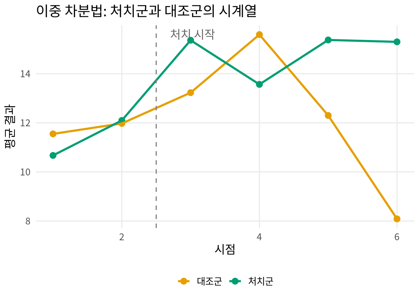
DiD의 주요 아이디어는 처치군에서 관찰된 변화에서 처치가 없었을 경우의 변화를 제외하는 것입니다. 대조군은 처치가 없었을 때의 반사실적 변화를 대신하는 역할을 합니다.

library(dplyr)
library(broom)
library(ggplot2)

# 확장된 DiD 예시: 여러 시점의 데이터
# 시나리오: 특정 지역에서 최저임금 인상 정책 도입
set.seed(42)
n_regions <- 20
n_time <- 6
treatment_time <- 3  # 3기에 처치 시작

did_panel <- expand.grid(
  region = 1:n_regions,
  time = 1:n_time
) |>
  tibble() |>
  mutate(
    # 처치군: 지역 11~20
    treated_region = as.integer(region > n_regions / 2),
    # 처치: 처치군에서 처치 시점 이후
    treatment = as.integer(treated_region == 1 & time >= treatment_time),
    # 지역 고정 효과
    region_fe = rep(rnorm(n_regions, 0, 2), each = n_time),
    # 공통 시간 추세
    time_trend = time * 0.5,
    # 결과 변수 (처치 효과 = 2.5)
    outcome = 10 + region_fe + time_trend + 2.5 * treatment +
      rnorm(n_regions * n_time, 0, 0.8)
  ) |>
  mutate(region = as.factor(region))

did_summary <- did_panel |>
  group_by(time, treated_region) |>
  summarize(mean_outcome = mean(outcome), .groups = "drop") |>
  mutate(group = ifelse(treated_region == 1, "처치군", "대조군"))

ggplot(did_summary, aes(x = time, y = mean_outcome,
                         color = group, group = group)) +
  geom_point(size = 3) +
  geom_line(linewidth = 1.2) +
  geom_vline(xintercept = treatment_time - 0.5,
             linetype = "dashed", color = "grey50") +
  annotate("text", x = treatment_time - 0.3, y = max(did_summary$mean_outcome),
           label = "처치 시작", hjust = 0, color = "grey40") +
  scale_color_manual(values = c("처치군" = "#009E73", "대조군" = "#E69F00")) +
  labs(
    x = "시점",
    y = "평균 결과",
    color = NULL,
    title = "이중 차분법: 처치군과 대조군의 시계열"
  )

그림 23.1: 이중 차분법의 평행 추세 가정 검증. 처치 시점 이전에 두 그룹의 추세가 평행해야 DiD 추정이 유효합니다.

23.1.2 TWFE(Two-Way Fixed Effects) 모델

전통적인 DiD는 이원 고정 효과(Two-Way Fixed Effects, TWFE) 모델로 추정됩니다:

\[Y_{it} = \alpha_i + \lambda_t + \delta D_{it} + \varepsilon_{it}\]

여기서: - \(\alpha_i\): 개인(지역) 고정 효과 - \(\lambda_t\): 시간 고정 효과 - \(D_{it}\): 처치 더미 (처치군 & 처치 이후 시점 = 1) - \(\delta\): DiD 추정치

# TWFE 모델 추정
# 지역과 시간 고정 효과를 factor로 처리
did_twfe <- lm(
  outcome ~ treatment + region + factor(time),
  data = did_panel
)

tidy(did_twfe) |>
  filter(term == "treatment")

# A tibble: 1 × 5
  term      estimate std.error statistic p.value
  <chr>        <dbl>     <dbl>     <dbl>   <dbl>
1 treatment     2.98      1.01      2.94 0.00414

# 또는 plm 패키지를 사용한 패널 데이터 분석
# install.packages("plm")
# library(plm)
# plm_did <- plm(
#   outcome ~ treatment,
#   data = did_panel,
#   index = c("region", "time"),
#   model = "within",   # 고정 효과
#   effect = "twoways"  # 이원 고정 효과
# )
# summary(plm_did)

# 이벤트 스터디(Event study): 각 시점별 효과 추정
event_study <- lm(
  outcome ~ treated_region * factor(time) + factor(time),
  data = did_panel
)

event_study_results <- tidy(event_study, conf.int = TRUE) |>
  filter(grepl("treated_region:factor\\(time\\)", term)) |>
  mutate(
    time = as.numeric(gsub("treated_region:factor\\(time\\)", "", term))
  ) |>
  bind_rows(
    tibble(term = "treated_region:factor(time)2",
           estimate = 0, conf.low = 0, conf.high = 0, time = 2)
  ) |>
  arrange(time)

ggplot(event_study_results, aes(x = time, y = estimate)) +
  geom_point(size = 3, color = "#009E73") +
  geom_errorbar(
    aes(ymin = conf.low, ymax = conf.high),
    width = 0.2, color = "#009E73"
  ) +
  geom_hline(yintercept = 0, linetype = "dashed") +
  geom_vline(xintercept = treatment_time - 0.5,
             linetype = "dotted", color = "grey50") +
  labs(
    x = "시점",
    y = "추정된 처치 효과 (ref: 시점 2)",
    title = "이벤트 스터디: 처치 효과의 동적 패턴"
  )

그림 23.2: 이벤트 스터디 플롯. 처치 시점(기간 3) 이전에는 효과가 0에 가까워야 하고(평행 추세 가정 검증), 처치 이후에는 처치 효과가 나타납니다.

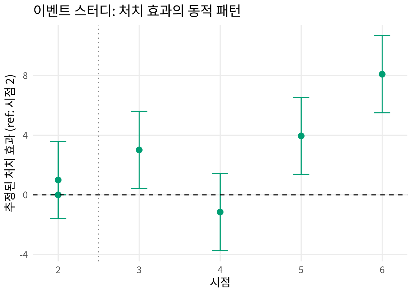
이벤트 스터디에서 처치 전 지점의 추정치가 0에 가까우면 평행 추세 가정에 대한 지지 근거가 됩니다.

23.1.3 이종적 처치 시점 문제 (Staggered adoption)

최근 계량경제학 연구는 TWFE 모델의 주요한 한계를 규명했습니다. 이종 처치 시점(staggered adoption) 설계의 TWFE 추정치는 음수 가중치가 부여된 처치 효과가 섞여 있어 해석하기 힘듭니다.

# 이종 처치 시점 예시
set.seed(2024)

staggered_data <- expand.grid(
  unit = 1:30,
  time = 1:8
) |>
  tibble() |>
  mutate(
    # 처치 시점이 다른 세 그룹
    treat_cohort = case_when(
      unit <= 10 ~ 3,   # 시점 3에 처치
      unit <= 20 ~ 5,   # 시점 5에 처치
      TRUE ~ Inf         # 처치 없음
    ),
    treatment = as.integer(time >= treat_cohort),
    unit_fe = rep(rnorm(30, 0, 1), each = 8),
    time_trend = time * 0.3,
    # 각 코호트마다 다른 처치 효과
    te = case_when(
      treat_cohort == 3 ~ 2,
      treat_cohort == 5 ~ 4,
      TRUE ~ 0
    ),
    outcome = 5 + unit_fe + time_trend + te * treatment + rnorm(30 * 8, 0, 0.5)
  )

# TWFE는 이 경우 편향될 수 있음
twfe_staggered <- lm(
  outcome ~ treatment + factor(unit) + factor(time),
  data = staggered_data
)

cat("TWFE 추정치 (이종 처치 시점에서 편향 가능):",
    round(tidy(twfe_staggered) |> filter(term == "treatment") |> pull(estimate), 3), "\n")

TWFE 추정치 (이종 처치 시점에서 편향 가능): 2.921 

cat("참 효과 (가중 평균):",
    round((2 * 10 + 4 * 10) / 20, 1), "\n")

참 효과 (가중 평균): 3 

이를 해결하기 위한 현대적 추정량으로는 Callaway & Sant’Anna(2021)의 방법이 있습니다:

# install.packages("did")
library(did)

# Callaway & Sant'Anna 이종 처치 시점 DiD
cs_did <- att_gt(
  yname = "outcome",
  tname = "time",
  idname = "unit",
  gname = "treat_cohort",
  data = staggered_data |> mutate(treat_cohort = ifelse(is.infinite(treat_cohort), 0, treat_cohort))
)

# 집계된 처치 효과
aggte(cs_did, type = "simple")

23.2 합성 대조군 (Synthetic controls)

합성 대조군(Synthetic Control Method, SCM)은 Abadie et al.(2010)이 개발한 방법으로, 처치된 단일 단위(국가, 지역 등)의 반사실적 결과를 대조군들의 가중 조합으로 구성합니다.

이 방법은 처치받지 않은 집단이 처치군을 비교하기에 적합하지 않을 때 특히 유용합니다.

# 합성 대조군 시뮬레이션
set.seed(2024)
n_donors <- 10
n_time <- 16
treat_time <- 8

# 대조군 단위들의 결과
donor_outcomes <- matrix(
  rnorm(n_donors * n_time, mean = 10, sd = 2),
  nrow = n_time, ncol = n_donors
) |>
  as.data.frame() |>
  setNames(paste0("donor_", 1:n_donors))

# 처치를 받은 단위의 결과 (대조군들의 가중 조합 + 처치 효과)
# 참 가중치: donor_1은 0.4, donor_2는 0.3, donor_3는 0.3
true_weights <- c(0.4, 0.3, 0.3, rep(0, n_donors - 3))
pre_treat_synthetic <- as.matrix(donor_outcomes[1:treat_time, ]) %*% true_weights

treated_unit <- c(
  pre_treat_synthetic + rnorm(treat_time, 0, 0.5),  # 처치 전 (합성 대조군과 유사)
  pre_treat_synthetic[treat_time] + (1:8) * 0.5 + 3 + rnorm(8, 0, 0.5)  # 처치 후 (효과 발생)
)

# 최적 가중치 찾기 (처치 전 기간에서 처치 단위와 유사하도록)
pre_treat_matrix <- as.matrix(donor_outcomes[1:treat_time, ])
pre_treat_treated <- treated_unit[1:treat_time]

# 최소제곱법으로 가중치 추정 (비음수 제약 포함은 생략하고 단순화)
sc_weights_fit <- lm(pre_treat_treated ~ pre_treat_matrix - 1)
sc_weights <- coef(sc_weights_fit)
sc_weights[sc_weights < 0] <- 0
sc_weights <- sc_weights / sum(sc_weights)

# 합성 대조군 구성
synthetic_control <- as.matrix(donor_outcomes) %*% sc_weights

synth_plot_data <- tibble(
  time = 1:n_time,
  treated = treated_unit,
  synthetic = as.numeric(synthetic_control)
) |>
  tidyr::pivot_longer(
    cols = c(treated, synthetic),
    names_to = "group",
    values_to = "outcome"
  ) |>
  mutate(
    group_label = ifelse(group == "treated", "처치 단위 (실제)", "합성 대조군")
  )

ggplot(synth_plot_data, aes(x = time, y = outcome,
                              color = group_label, linetype = group_label)) +
  geom_line(linewidth = 1.2) +
  geom_vline(xintercept = treat_time + 0.5,
             linetype = "dashed", color = "grey50") +
  annotate("text", x = treat_time + 1, y = max(treated_unit),
           label = "처치 시작", hjust = 0, color = "grey40") +
  scale_color_manual(values = c("처치 단위 (실제)" = "#009E73",
                                 "합성 대조군" = "#E69F00")) +
  scale_linetype_manual(values = c("처치 단위 (실제)" = "solid",
                                    "합성 대조군" = "dashed")) +
  labs(
    x = "시점",
    y = "결과",
    color = NULL,
    linetype = NULL,
    title = "합성 대조군: 처치 효과 추정"
  )

Warning: Removed 16 rows containing missing values or values
outside the scale range (`geom_line()`).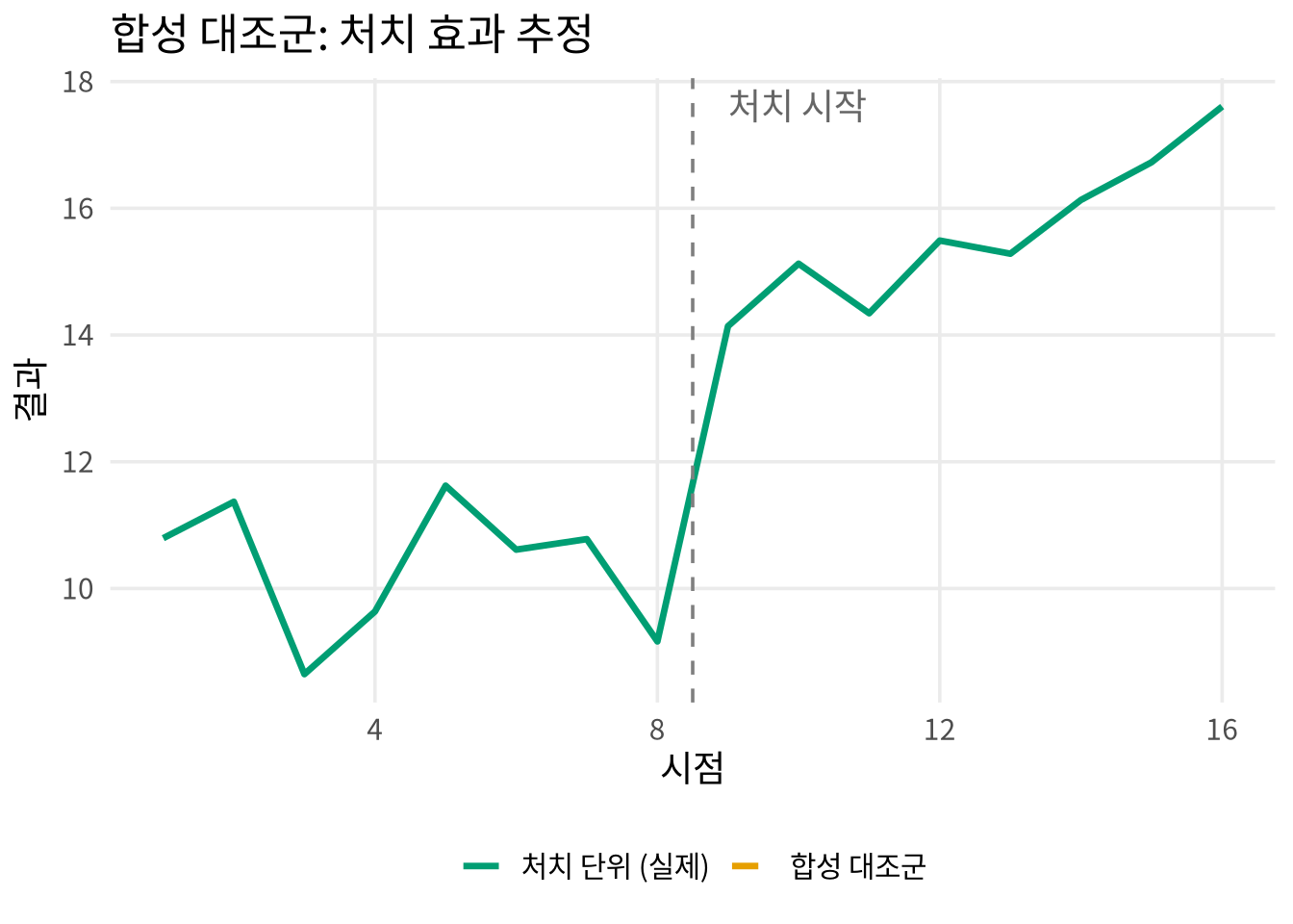

그림 23.3: 합성 대조군 방법의 시각화. 실선은 처치를 받은 단위의 실제 결과이고, 점선은 대조군들의 가중 조합으로 구성된 합성 대조군의 추세입니다. 처치 후의 두 선 간의 차이가 처치 효과 추정치입니다.

합성 대조군 방법의 처치 효과는 처치 후 실제 결과와 합성 대조군의 차이로 계산합니다. 추론에는 치환 검정(permutation tests) 또는 플라세보 검정(placebo tests)을 사용합니다.

노트DiD vs. 합성 대조군

특성	DiD	합성 대조군
처치 단위 수	여러 단위 가능	보통 1~수 개
대조군 수	적어도 됨	많을수록 좋음
식별 가정	평행 추세	처치 전 기간 적합
추론 방법	표준 회귀 추론	치환 검정
적용 예시	정책 평가	자연 실험, 사례 연구

두 방법 모두 시계열 데이터에서 인과 효과를 추정하는 강력한 도구이므로, 연구 설계와 데이터 구조에 맞춰 적합한 방법을 선택해야 합니다.