# pip install --pre pycaret
!pip install -U pycaret -qPyCaret 설치
Google Colab 사용자의 경우 다음의 코드를 실행합니다.
from pycaret.utils import enable_colab

enable_colab()
분류 Classification
분류 모델은 정답 값(label)에 대하여 클래스(class)가 존재하면 개별 데이터를 특정 클래스로 분류할 수 있는 모델입니다.
(예시) 암/정상 환자 분류, 스팸/햄 메일 분류
필요한 모듈 import
import pandas as pd
import numpy as np
import seaborn as sns

pd.options.display.max_columns = None
실습을 위한 데이터셋 로드
from IPython.display import Image

Image('https://static1.squarespace.com/static/5006453fe4b09ef2252ba068/t/5090b249e4b047ba54dfd258/1351660113175/TItanic-Survival-Infographic.jpg')
건조 당시 세계 최대의 여객선이었지만,1912년의 최초이자 최후의 항해 때 빙산과 충돌해 침몰한 비운의 여객선. 아마도 세상에서 가장 유명한 여객선이자 침몰선일 것입니다.
침몰한 지 100년이 넘었지만 아직까지 세계에서 가장 유명한 침몰선입니다.
사망자 수는 1위는 아니지만, 세계적으로 유명한 영화의 영향도 있고, 당시 최첨단 기술에 대해 기대감이 컸던 사회에 큰 영향을 끼치기도 한데다가, 근대 사회에서 들어서자마자 얼마 안된, 그리고 유명인사들이 여럿 희생된 대참사이기 때문에 가장 유명한 침몰선이 되었습니다. 또한 이 사건을 기점으로 여러가지 안전 조약들이 생겨났으니 더더욱 그렇습니다.
dataset = sns.load_dataset('titanic')
dataset.head()
# 데이터셋 크기 출력
dataset.shape컬럼 설명
- survivied: 생존여부 (1: 생존, 0: 사망)
- pclass: 좌석 등급 (1등급, 2등급, 3등급)
- sex: 성별
- age: 나이
- sibsp: 형제 + 배우자 수
- parch: 부모 + 자녀 수
- fare: 좌석 요금
- embarked: 탑승 항구 (S, C, Q)
- class: pclass와 동일
- who: 성인남자(man), 성인여자(woman), 어린아이(child)
- adult_male: 성인 남자 여부
- deck: 데크 번호 (알파벳 + 숫자 혼용)
- embark_town: 탑승 항구 이름
- alive: 생존여부 (yes, no)
- alone: 혼자 탑승 여부
PyCaret의 큰 구조
- STEP1: initialize
- STEP2: train
- STEP3: optimize
- STEP4: analyze
- STEP5: deploy
셋업 setup()
분류 예측 모형(Classification Model)을 생성하기 위한 첫 단계로 다음을 import 합니다.
from pycaret.classification import * # 분류setup 함수
data: 학습할 데이터셋을 지정합니다.target: 분류 예측할 대상(target) 컬럼을 지정합니다.session_id: SEED 값을 지정합니다.
setup() 함수 실행시 AutoML / 데이터 전처리시 적용할 다양한 옵션 값들을 출력합니다.
clf = setup(data=dataset,
            target='survived',
            session_id=123,
) verbose: default=True. False로 설정시 설정에 대한 출력생성을 생략합니다.
clf = setup(data=dataset,
            target='survived',
            session_id=123,
            verbose=False, # False로 설정시 설정에 대한 출력생성을 생략합니다. (default=True)
           )
모든 모델에 대한 학습: compare_models()
compare_models - sort: 정렬 기준이 되는 평가지표를 설정합니다. - n_select: 상위 N개의 알고리즘을 선택합니다. - fold: Cross Validation 평가 Fold의 개수를 지정합니다.
best_model = compare_models(sort='Accuracy', n_select=3, fold=5)# 제일 성능이 좋은 모델을 출력합니다.
print(best_model)survived를 예측하는 정확도가 상당히 높게 나왓습니다.
alive 컬럼이 dataset에 속해 있기 때문에 머신러닝 알고리즘이 alive컬럼 정보를 보고 예측했을 가능성이 큽니다.
따라서, alive 컬럼을 제거한 후 다시 머신러닝 학습 모델을 만들어 보도록 하겠습니다.
dataset.head(3)ignore_features에 리스트(list) 형식으로 컬럼 정보를 지정합니다. 이 옵션에 지정된 컬럼 정보는 분석 / 학습시 무시하게 됩니다.verbose=False는 컬럼 정보가 맞게 설정이 되었는지 확인차 다시 물어보는 interactive 창을 띄우지 않습니다.
clf = setup(data=dataset,
            ignore_features=['alive'], # 분석/학습에 고려하지 않을 feature(컬럼) 제거
            target='survived',
            session_id=123,
            verbose=False,
            )
best_model = compare_models(sort='Accuracy', n_select=3, fold=5)컬럼의 특성 세부 정의
setup 함수
data: 학습할 데이터셋을 지정합니다.target: 예측할 대상(target) 컬럼을 지정합니다.session_id: SEED 값을 지정합니다.profile: True로 설정시 데이터 프로파일링을 출력합니다.
ignore_features에는 분석 / 학습에 무시할 컬럼을 지정합니다.
alive,embark_town,class는 다른 컬럼과 겹치는 컬럼이므로 제외합니다.
ignore_features=['alive', 'embark_town', 'class']dataset[ignore_features].head()categorical_features에는 범주형 컬럼을 지정합니다. - pclass, sex, embarked 컬럼은 범주형 특성을 가집니다. 즉, 카테고리화 할 수 있는 컬럼을 의미합니다.
categorical_features=['sex', 'embarked', 'who', 'deck']dataset[categorical_features].head()ordinal_features에는 순서형 특성을 가진 컬럼을 대입합니다.
예를 들어, ‘low’, ‘medium’, ’high’의 값을 가지는데 low < medium < high표현될 수 있다면
ordinal_features = {'column_name' : ['low', 'medium', 'high']} 와 같이 대입할 수 있습니다.
ordinal_features = {
    'pclass': [1, 2, 3]
}numeric_features에는 수치형 컬럼을 지정합니다. - age, fare, sibsp, parch는 숫자형태의 데이터를 가지므로 수치형 컬럼에 지정합니다.
numeric_features=['age', 'fare', 'sibsp', 'parch']dataset[numeric_features].head()clf = setup(data=dataset,
target='survived',
ignore_features=ignore_features, # 분석/학습에 고려하지 않을 feature(컬럼) 제거
categorical_features=categorical_features, # 범주형 컬럼 지정
numeric_features=numeric_features, # 수치형 컬럼 지정
ordinal_features=ordinal_features,
session_id=123,
verbose=False,
) 고급 전처리 전략
- [참고] 도큐먼트 (링크)
결측치 채우기
imputation_type: ‘simple’ or ‘iterative’, default = ‘simple’numeric_imputation: int, float or str, default = ‘mean’categorical_imputation: str, default = ‘constant’
imputation_type은 simple과 iterative 중 택할 수 있으며, 기본 값은 simple로 설정되어 있습니다.
simple일 경우 단순 통계량이나 고정된 값으로 결측치를 채웁니다.
하지만 iterative로 설정된 경우 머신러닝 알고리즘 (대표적으로 lightgbm)으로 예측된 값이 채워지게 됩니다.
imputation_type='iterative'으로 설정된 경우 다음의 Value설정 값은 무시됩니다.
numeric_imputation - “drop”: Drop rows containing missing values. - “mean”: Impute with mean of column. - “median”: Impute with median of column. - “mode”: Impute with most frequent value. - “knn”: Impute using a K-Nearest Neighbors approach. - int or float: Impute with provided numerical value.
categorical_imputation - “drop”: Drop rows containing missing values. - “mode”: Impute with most frequent value. - str: Impute with provided string.
예시 1)
clf = setup(data=dataset,
            target='survived',
            ignore_features=ignore_features,           # 분석/학습에 고려하지 않을 feature(컬럼) 제거
            categorical_features=categorical_features, # 범주형 컬럼 지정
            numeric_features=numeric_features,         # 수치형 컬럼 지정
            ordinal_features=ordinal_features,         # 순서형 컬럼 지정
            imputation_type='iterative',               # 예측하여 결측치를 보간하는 경우
            session_id=123,
            verbose=False,
            )
예시 2)
clf = setup(data=dataset,
            target='survived',
            ignore_features=ignore_features,           # 분석/학습에 고려하지 않을 feature(컬럼) 제거
            categorical_features=categorical_features, # 범주형 컬럼 지정
            numeric_features=numeric_features,         # 수치형 컬럼 지정
            ordinal_features=ordinal_features,         # 순서형 컬럼 지정
            imputation_type='simple',                  # 고정된 값으로 결측치를 보간하는 경우
            numeric_imputation='median',
            categorical_imputation='mode',
            session_id=123,
            verbose=False,
            )
정규화 방법 정의
normalize / normalize_method
normalize: bool, default = Falsenormalize_method: str, default = ‘zscore’
normalize는 데이터의 정규화/표준화 여부를 설정합니다.
normalize_method는 기본 ’zscore’가 설정되어 있습니다.
- ‘minmax’: scales and translates each feature individually such that it is in the range of 0 - 1.
- ‘maxabs’: scales and translates each feature individually such that the maximal absolute value of each feature will be 1.0.
- ‘robust’: scales and translates each feature according to the Interquartile range. When the dataset contains outliers, robust scaler often gives better results.
clf = setup(data=dataset,
            target='survived',
            ignore_features=ignore_features,           # 분석/학습에 고려하지 않을 feature(컬럼) 제거
            categorical_features=categorical_features, # 범주형 컬럼 지정
            numeric_features=numeric_features,         # 수치형 컬럼 지정
            ordinal_features=ordinal_features,         # 순서형 컬럼 지정
            imputation_type='simple',                  # 고정된 값으로 결측치를 보간하는 경우
            numeric_imputation='median',
            categorical_imputation='mode',
            normalize=True,
            normalize_method='zscore',
            session_id=123,
            verbose=False,
            )
다수 모델의 학습 및 블렌딩: compare_models(), blend_models()
모든 알고리즘에 대하여 학습 결과 비교: compare_models()
sort: 정렬 기준이 되는 평가지표를 설정합니다.n_select: 상위 N개의 알고리즘을 선택합니다.fold: Cross Validation 평가 Fold의 개수를 지정합니다.
best_models = compare_models(sort='Accuracy', n_select=3, fold=5)가장 좋은 결과를 낸 모델을 블렌딩: blend_models()
compare_models로 추출된 best 모델에 대하여 모델 블렌딩하여 성능 개선Softvote 방식으로estimator_list에 적용된 모델을 앙상블Voting Ensemble: 투표를 통해 결과 도출
Voting은 단어 뜻 그대로 투표를 통해 결정하는 방식입니다.
Voting에는 크게 2가지로 투표 방식이 나뉩니다. (hard / soft)
hard vote 방식에서는 결과 값에 대한 다수 class를 차용합니다.
classification을 예로 들어 보자면, 분류를 예측한 값이 1, 0, 0, 1, 1 이었다고 가정한다면 1이 3표, 0이 2표를 받았기 때문에 Hard Voting 방식에서는 1이 최종 값으로 예측을 하게 됩니다.
soft vote 방식은 각각의 확률의 평균 값을 계산한다음에 가장 확률이 높은 값으로 확정짓게 됩니다.
가령 class 0이 나올 확률이 (0.4, 0.9, 0.9, 0.4, 0.4)이었고, class 1이 나올 확률이 (0.6, 0.1, 0.1, 0.6, 0.6) 이었다면,
- class 0이 나올 최종 확률은 (0.4+0.9+0.9+0.4+0.4) / 5 = 0.44,
- class 1이 나올 최종 확률은 (0.6+0.1+0.1+0.6+0.6) / 5 = 0.4
가 되기 때문에 앞선 Hard Vote의 결과와는 다른 결과 값이 최종 으로 선출되게 됩니다.
blended_models = blend_models(best_models, fold=5)단일 모델 생성: create_model()
먼저, 학습 가능한 모델의 리스트를 출력합니다.
models()출력된 모델 중 하나의 알고리즘을 선택하여 생성합니다.
dt: decision tree 알고리즘
dt = create_model('dt')# decision tree 알고리즘의 세부 설정 옵션에 대한 내용을 확인할 수 있습니다.
dt다음과 같이 생성시 사용자 정의 학습 파라미터 설정도 가능합니다.
# max_depth=5로 설정시
dt = create_model('dt', max_depth=5)dtpull() 함수로 모델의 학습 결과를 DataFrame으로 가져올 수 있습니다.
# 학습 결과를 dt_result에 저장
dt_result = pull()
dt_result
단일 모델에 대한 앙상블: ensemble_model()
단일 모델에 대한 앙상블 방식은 Bagging 방식을 사용합니다.
Bagging 앙상블 자세한 내용 보기 (링크)
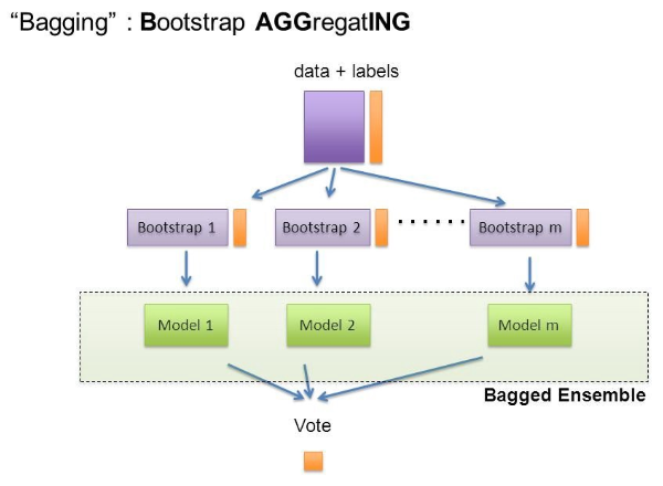
Bagging은 Bootstrap Aggregating의 줄임말입니다.
- Bootstrap = Sample(샘플) + Aggregating = 합산
Bootstrap은 여러 개의 dataset을 중첩을 허용하게 하여 샘플링하여 분할하는 방식
데이터 셋의 구성이 [1, 2, 3, 4, 5 ]로 되어 있다면,
- group 1 = [1, 2, 3]
- group 2 = [1, 3, 4]
- group 3 = [2, 3, 5]
dt = create_model('dt')
bagged_dt = ensemble_model(dt)
Boosting 앙상블 자세한 내용 보기 (링크)
Boosting 알고리즘 역시 앙상블 학습 (ensemble learning)이며, 약한 학습기를 순차적으로 학습을 하되, 이전 학습에 대하여 잘못 예측된 데이터에 가중치를 부여해 오차를 보완해 나가는 방식입니다.
다른 앙상블 기법과 가장 다른 점중 하나는 바로 순차적인 학습을 하며 weight를 부여해서 오차를 보완해 나간다는 점인데요. 순차적이기 때문에 병렬 처리에 어려움이 있고, 그렇기 때문에 다른 앙상블 대비 학습 시간이 오래걸린다는 단점이 있습니다.
dt = create_model('dt')
# boosting 방식 적용시
boosted_dt = ensemble_model(dt, method = 'Boosting')
기본적으로 PyCaret은 Bagging 또는 Boosting 모두에 10개의 추정기를 사용합니다. n_estimators 매개 변수를 변경하여 이 값을 증가시킬 수 있습니다.
dt = create_model('dt')
# boosting 방식 적용시
bagged_dt = ensemble_model(dt, n_estimators=200, choose_better=True)
calibrate_model()
이 함수는 isotonic 또는 로지스틱 회귀 분석을 사용하여 주어진 모형의 확률을 보정합니다. 이 함수의 출력은 폴드별 CV 점수를 가진 스코어링 그리드입니다. CV 중에 평가된 메트릭은 get_metrics 함수를 사용하여 액세스할 수 있습니다.
calibrated_dt = calibrate_model(bagged_dt)예측: predict_model()
# 예측
result = predict_model(estimator=bagged_dt)result[['survived','Label', 'Score']]예측용 데이터셋으로 예측한 경우
# 랜덤하게 100개 추출
unseen_data = dataset.sample(100)
# unseen data 대입
result = predict_model(data=unseen_data, estimator=bagged_dt)finalize_model()
- 이 단계에서는 전체 데이터셋을 활용하여 재학습을 진행합니다.
# finalize a model
final_model = finalize_model(bagged_dt)
모델 저장 및 로드
학습이 완료된 모델을 저장합니다.
# save config
save_config('myconfig-01')

# save pipeline
save_model(final_model, 'mymodel-01')
저장한 모델을 다시 로드하는 경우
load_config('myconfig-01')

# load pipeline
loaded_model = load_model('mymodel-01')