import pandas as pd
import numpy as np7장: 팬더 소개

학습 내용
학습 목표
pd.Series()를 사용하여 Pandas 시리즈를 만들고pd.DataFrame()을 사용하여 Pandas 데이터프레임을 만듭니다.df[],df.loc[],df.iloc[],df.query[]와 같은 표기법을 사용하여 인덱싱, 슬라이싱 및 불리언(Boolean) 인덱싱을 통해 시리즈/데이터 프레임의 값에 액세스할 수 있습니다.- 두 계열 간의 기본 산술 연산을 수행하고 결과를 예상합니다.
- Pandas가 dtype을 Series에 할당하는 방법과
objectdtype이 무엇인지 설명 - Pandas
pd.read_csv()를 사용하여 로컬 경로 또는 URL에서 표준 .csv 파일을 읽습니다. - Python에서
np.ndarray,pd.Series및pd.DataFrame개체 간의 관계와 차이점을 설명합니다.
1. 팬더 소개

Pandas는 테이블 형식 데이터 구조에 가장 널리 사용되는 Python 라이브러리입니다. Pandas는 매우 강력한 Excel 버전이라고 생각할 수 있습니다(그러나 무료이며 훨씬 더 많은 함수을 제공합니다!).
Pandas는 conda를 사용하여 설치할 수 있습니다.
콘다 설치 팬더우리는 일반적으로 pd라는 별칭을 사용하여 팬더를 가져옵니다. 대부분의 데이터 과학 워크플로 상단에 다음 두 가지 가져오기가 표시됩니다.
2. 팬더 시리즈
시리즈란 무엇인가요?
Series는 NumPy 배열과 비슷하지만 레이블이 있습니다. 이는 엄격히 1차원이며 혼합을 포함하여 모든 데이터 타입(정수, 문자열, 부동 소수점, 객체 등)을 포함할 수 있습니다. 시리즈는 pd.Series()를 사용하여 스칼라, 리스트, ndarray 또는 딕셔너리에서 생성될 수 있습니다(대문자 “S”에 유의하세요). 다음은 몇 가지 예시 시리즈입니다.
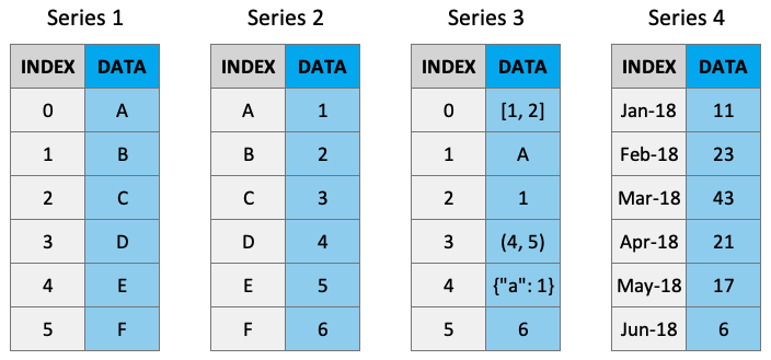
시리즈 만들기
기본적으로 계열에는 0부터 시작하는 인덱스로 레이블이 지정됩니다. 예를 들면 다음과 같습니다.
pd.Series(data=[-5, 1.3, 21, 6, 3])0 -5.0
1 1.3
2 21.0
3 6.0
4 3.0
dtype: float64하지만 사용자 정의 색인을 추가할 수 있습니다.
pd.Series(data=[-5, 1.3, 21, 6, 3], index=["a", "b", "c", "d", "e"])a -5.0
b 1.3
c 21.0
d 6.0
e 3.0
dtype: float64딕셔너리에서 시리즈를 만들 수 있습니다.
pd.Series(data={"a": 10, "b": 20, "c": 30})a 10
b 20
c 30
dtype: int64또는 ndarray에서:
pd.Series(data=np.random.randn(3)) # noqa: F405, F811, F8210 -0.428301
1 -0.104959
2 0.170835
dtype: float64또는 스칼라일 수도 있습니다:
pd.Series(3.141)0 3.141
dtype: float64pd.Series(data=3.141, index=["a", "b", "c"])a 3.141
b 3.141
c 3.141
dtype: float64시리즈 특성
시리즈에는 name 속성을 부여할 수 있습니다. 나는 이것을 거의 사용하지 않지만 가끔 나타날 수 있습니다.
s = pd.Series(data=np.random.randn(5), name="random_series")  # noqa: F405, F811, F821
s
0 -1.363190
1 0.425801
2 -0.048966
3 -0.298172
4 1.899199
Name: random_series, dtype: float64s.name'random_series's.rename("another_name")0 -1.363190
1 0.425801
2 -0.048966
3 -0.298172
4 1.899199
Name: another_name, dtype: float64.index 속성을 사용하여 시리즈의 색인 라벨에 액세스할 수 있습니다.
s.indexRangeIndex(start=0, stop=5, step=1).to_numpy()를 사용하여 기본 데이터 배열에 액세스할 수 있습니다.
s.to_numpy()array([-1.36319006, 0.42580052, -0.04896627, -0.29817227, 1.89919866])pd.Series([[1, 2, 3], "b", 1]).to_numpy()array([list([1, 2, 3]), 'b', 1], dtype=object)인덱싱 및 슬라이싱 시리즈
시리즈는 ndarray와 매우 유사합니다(실제로 시리즈는 대부분의 NumPy 함수에 전달될 수 있습니다!). 대괄호 [ ]를 사용하여 색인을 생성하고 콜론 : 표기법을 사용하여 분할할 수 있습니다.
s = pd.Series(data=range(5), index=["A", "B", "C", "D", "E"])  # noqa: F811
s
A 0
B 1
C 2
D 3
E 4
dtype: int64s[0]0s[[1, 2, 3]]B 1
C 2
D 3
dtype: int64s[0:3]A 0
B 1
C 2
dtype: int64위에서 배열 기반 인덱싱 및 슬라이싱이 시리즈 인덱스를 반환하는 방법을 참고하세요.
시리즈는 인덱스 레이블을 사용하여 값에 액세스할 수 있다는 점에서 딕셔너리과 비슷합니다.
s["A"]0s[["B", "D", "C"]]B 1
D 3
C 2
dtype: int64s["A":"C"]A 0
B 1
C 2
dtype: int64"A" in sTrue"Z" in sFalse시리즈는 고유하지 않은 인덱싱을 허용하지만 인덱싱 작업은 고유한 값을 반환하지 않으므로 주의하세요.
x = pd.Series(data=range(5), index=["A", "A", "A", "B", "C"]) # noqa: F811
xA 0
A 1
A 2
B 3
C 4
dtype: int64x["A"]A 0
A 1
A 2
dtype: int64마지막으로 시리즈를 사용하여 불리언(Boolean) 인덱싱을 수행할 수도 있습니다.
s[s >= 1]B 1
C 2
D 3
E 4
dtype: int64s[s > s.mean()]D 3
E 4
dtype: int64(s != 1)A True
B False
C True
D True
E True
dtype: bool시리즈 운영
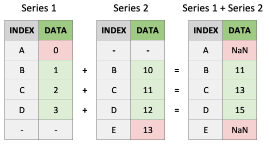
Series(+, -, /, *) 간의 ndarrays 작업과 달리 LABELS(구조에서의 위치가 아님)를 기준으로 값을 정렬합니다. 결과 인덱스는 두 인덱스의 __정렬된 합집합__이 됩니다. 이를 통해 레이블에 관계없이 시리즈 작업을 실행할 수 있는 유연성이 제공됩니다.
s1 = pd.Series(data=range(4), index=["A", "B", "C", "D"]) # noqa: F811
s1A 0
B    1
C    2
D    3
dtype: int64s2 = pd.Series(data=range(10, 14), index=["B", "C", "D", "E"]) # noqa: F811
s2B 10
C 11
D 12
E 13
dtype: int64s1 + s2A NaN
B 11.0
C 13.0
D 15.0
E NaN
dtype: float64위에서 볼 수 있듯이 일치하는 인덱스가 연산됩니다. 일치하지 않는 인덱스는 제품에 표시되지만 ‘NaN’ 값과 함께 표시됩니다.
안타깝게도 해당 사용자는 다음 작업을 수행할 수 없습니다.
s1**2A 0
B 1
C 4
D 9
dtype: int64np.exp(s1)A 1.000000
B 2.718282
C 7.389056
D 20.085537
dtype: float64마지막으로, 배열과 마찬가지로 시리즈에는 다양한 작업을 위한 많은 내장 메서드가 있습니다. help(pd.Series)를 실행하여 모두 찾을 수 있습니다.
print([_ for _ in dir(pd.Series) if not _.startswith("_")]) # print all common methods['T', 'abs', 'add', 'add_prefix', 'add_suffix', 'agg', 'aggregate', 'align', 'all', 'any', 'append', 'apply', 'argmax', 'argmin', 'argsort', 'array', 'asfreq', 'asof', 'astype', 'at', 'at_time', 'attrs', 'autocorr', 'axes', 'backfill', 'between', 'between_time', 'bfill', 'bool', 'cat', 'clip', 'combine', 'combine_first', 'compare', 'convert_dtypes', 'copy', 'corr', 'count', 'cov', 'cummax', 'cummin', 'cumprod', 'cumsum', 'describe', 'diff', 'div', 'divide', 'divmod', 'dot', 'drop', 'drop_duplicates', 'droplevel', 'dropna', 'dt', 'dtype', 'dtypes', 'duplicated', 'empty', 'eq', 'equals', 'ewm', 'expanding', 'explode', 'factorize', 'ffill', 'fillna', 'filter', 'first', 'first_valid_index', 'floordiv', 'ge', 'get', 'groupby', 'gt', 'hasnans', 'head', 'hist', 'iat', 'idxmax', 'idxmin', 'iloc', 'index', 'infer_objects', 'interpolate', 'is_monotonic', 'is_monotonic_decreasing', 'is_monotonic_increasing', 'is_unique', 'isin', 'isna', 'isnull', 'item', 'items', 'iteritems', 'keys', 'kurt', 'kurtosis', 'last', 'last_valid_index', 'le', 'loc', 'lt', 'mad', 'map', 'mask', 'max', 'mean', 'median', 'memory_usage', 'min', 'mod', 'mode', 'mul', 'multiply', 'name', 'nbytes', 'ndim', 'ne', 'nlargest', 'notna', 'notnull', 'nsmallest', 'nunique', 'pad', 'pct_change', 'pipe', 'plot', 'pop', 'pow', 'prod', 'product', 'quantile', 'radd', 'rank', 'ravel', 'rdiv', 'rdivmod', 'reindex', 'reindex_like', 'rename', 'rename_axis', 'reorder_levels', 'repeat', 'replace', 'resample', 'reset_index', 'rfloordiv', 'rmod', 'rmul', 'rolling', 'round', 'rpow', 'rsub', 'rtruediv', 'sample', 'searchsorted', 'sem', 'set_axis', 'shape', 'shift', 'size', 'skew', 'slice_shift', 'sort_index', 'sort_values', 'sparse', 'squeeze', 'std', 'str', 'sub', 'subtract', 'sum', 'swapaxes', 'swaplevel', 'tail', 'take', 'to_clipboard', 'to_csv', 'to_dict', 'to_excel', 'to_frame', 'to_hdf', 'to_json', 'to_latex', 'to_list', 'to_markdown', 'to_numpy', 'to_period', 'to_pickle', 'to_sql', 'to_string', 'to_timestamp', 'to_xarray', 'tolist', 'transform', 'transpose', 'truediv', 'truncate', 'tshift', 'tz_convert', 'tz_localize', 'unique', 'unstack', 'update', 'value_counts', 'values', 'var', 'view', 'where', 'xs']s1A 0
B 1
C 2
D 3
dtype: int64s1.mean()1.5s1.sum()6s1.astype(float)A 0.0
B 1.0
C 2.0
D 3.0
dtype: float64“체인 연결” 작업은 팬더에서도 일반적입니다.
s1.add(3.141).pow(2).mean().astype(int)22데이터 타입
Series는 int, float, bool 등과 같이 익숙한 모든 데이터 타입(dtypes)을 보유할 수 있습니다. 이 장과 이후 장에서 설명할 몇 가지 다른 특수 데이터 타입(object, DateTime 및 Categorical)도 있습니다. pandas dtypes에 대한 자세한 내용은 문서에서도 언제든지 읽을 수 있습니다. 예를 들어, 다음은 일련의 dtype int64입니다.
x = pd.Series(range(5))  # noqa: F811
x.dtypedtype('int64')dtype “object”는 일련의 문자열 또는 혼합 데이터에 사용됩니다. Pandas는 전용 문자열 dtype StringDtype을 사용하여 현재 실험 중이지만 아직 테스트 중입니다.
x = pd.Series(["A", "B"])  # noqa: F811
x
0 A
1 B
dtype: objectx = pd.Series(["A", 1, ["I", "AM", "A", "LIST"]]) # noqa: F811
x0 A
1 1
2 [I, AM, A, LIST]
dtype: object유연하지만 메모리 요구 사항이 높기 때문에 object dtype을 사용하지 않는 것이 좋습니다. 기본적으로 object dtype 시리즈에서 모든 단일 요소는 개별 dtype에 대한 정보를 저장합니다. 여러 가지 방법으로 혼합 계열에 있는 모든 요소의 dtype을 검사할 수 있습니다. 아래에서는 ‘map’ 메서드를 사용하겠습니다.
x.map(type)0 <class 'str'>
1 <class 'int'>
2 <class 'list'>
dtype: object시리즈의 각 객체에는 서로 다른 dtype이 있음을 알 수 있습니다. 여기에는 비용이 듭니다. 아래 시리즈의 메모리 사용량을 비교해 보세요.
x1 = pd.Series([1, 2, 3])  # noqa: F811
print(f"x1 dtype: {x1.dtype}")
print(f"x1 memory usage: {x1.memory_usage(deep=True)} bytes")
print("")
x2 = pd.Series([1, 2, "3"])  # noqa: F811
print(f"x2 dtype: {x2.dtype}")
print(f"x2 memory usage: {x2.memory_usage(deep=True)} bytes")
print("")
x3 = pd.Series([1, 2, "3"]).astype(
    "int8"
)  # coerce the object series to int8  # noqa: F811
print(f"x3 dtype: {x3.dtype}")
print(f"x3 memory usage: {x3.memory_usage(deep=True)} bytes")
x1 dtype: int64
x1 memory usage: 152 bytes
x2 dtype: object
x2 memory usage: 258 bytes
x3 dtype: int8
x3 memory usage: 131 bytes요약하자면, 가능하면 균일한 dtype을 사용하십시오. 메모리 효율성이 더 좋습니다!
또 하나의 문제인 NaN(데이터의 누락된 값을 나타내는 데 자주 사용됨)은 부동 소수점입니다.
type(np.NaN)floatPandas가 전체 계열을 부동소수점으로 변환하기 때문에 일련의 정수와 하나의 누락된 값이 있는 경우 문제가 될 수 있습니다.
pd.Series([1, 2, 3, np.NaN])0 1.0
1 2.0
2 3.0
3 NaN
dtype: float64최근에야 Pandas는 dtype에 영향을 주지 않고 정수 계열의 NaN을 처리할 수 있는 “nullable 정수 dtype”을 구현했습니다. 아래 유형의 대문자 “I”는 numpy의 int64 dtype과 구별됩니다.
pd.Series([1, 2, 3, np.NaN]).astype("Int64")0 1
1 2
2 3
3 <NA>
dtype: Int64이는 아직 Pandas의 기본값이 아니며 이 새로운 함수의 함수은 계속 변경될 수 있습니다.
3. 팬더 데이터프레임
데이터프레임이란 무엇인가요?
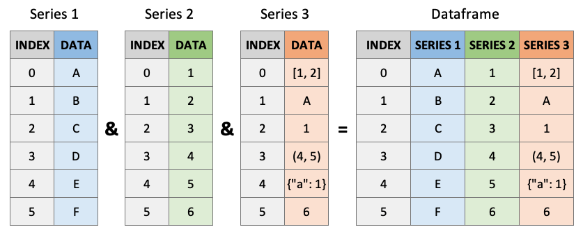
Pandas DataFrames는 당신의 새로운 절친한 친구입니다. 이는 익숙한 Excel 스프레드시트와 같습니다. DataFrame은 실제로 시리즈가 서로 붙어 있는 것입니다! DataFrame을 시리즈 딕셔너리으로 생각하세요. “키”는 열 레이블이고 “값”은 시리즈 데이터입니다.
데이터프레임 생성
데이터프레임은 pd.DataFrame()을 사용하여 생성할 수 있습니다(대문자 “D” 및 “F” 참고). 시리즈와 마찬가지로 데이터 프레임의 인덱스 및 열 레이블은 기본적으로 0부터 시작하여 레이블이 지정됩니다.
pd.DataFrame([[1, 2, 3], [4, 5, 6], [7, 8, 9]])| 0 | 1 | 2 | |
|---|---|---|---|
| 0 | 1 | 2 | 3 |
| 1 | 4 | 5 | 6 |
| 2 | 7 | 8 | 9 |
‘index’ 및 ‘columns’ 인수를 사용하여 라벨을 지정할 수 있습니다.
pd.DataFrame(
    [[1, 2, 3], [4, 5, 6], [7, 8, 9]],
    index=["R1", "R2", "R3"],  # noqa: F811
    columns=["C1", "C2", "C3"],  # noqa: F811
)| C1 | C2 | C3 | |
|---|---|---|---|
| R1 | 1 | 2 | 3 |
| R2 | 4 | 5 | 6 |
| R3 | 7 | 8 | 9 |
괄호는 생략될 수 있으며(종종 생략됨), ’튜플’은 쉼표를 사용하여 정의된 대로 암시적으로 반환됩니다.
pd.DataFrame({"C1": [1, 2, 3], "C2": ["A", "B", "C"]}, index=["R1", "R2", "R3"])| C1 | C2 | |
|---|---|---|
| R1 | 1 | A |
| R2 | 2 | B |
| R3 | 3 | C |
pd.DataFrame(
    np.random.randn(5, 5),  # noqa: F405, F811, F821
    index=[f"row_{_}" for _ in range(1, 6)],  # noqa: F811
    columns=[f"col_{_}" for _ in range(1, 6)],  # noqa: F811
)| col_1 | col_2 | col_3 | col_4 | col_5 | |
|---|---|---|---|---|---|
| row_1 | -1.511598 | -1.073875 | 2.990474 | 2.408082 | 0.101569 |
| row_2 | 0.767246 | 0.423030 | -0.135450 | 0.369545 | 0.761417 |
| row_3 | 0.714677 | 1.489430 | 0.843088 | -1.284666 | 1.310033 |
| row_4 | -0.513656 | 0.539531 | 0.207057 | 0.425888 | 0.481794 |
| row_5 | -1.361988 | -0.479158 | 0.158281 | -0.196813 | 0.136745 |
pd.DataFrame(np.array([["Tom", 7], ["Mike", 15], ["Tiffany", 3]]))| 0 | 1 | |
|---|---|---|
| 0 | Tom | 7 |
| 1 | Mike | 15 |
| 2 | Tiffany | 3 |
다음은 데이터프레임을 생성할 수 있는 주요 방법에 대한 표입니다(자세한 내용은 Pandas 설명서 참조).
| 다음에서 DataFrame 생성 | 코드 |
|---|---|
| 리스트 리스트 | pd.DataFrame([['Tom', 7], ['Mike', 15], ['Tiffany', 3]]) |
| ndarray | pd.DataFrame(np.array([['Tom', 7], ['Mike', 15], ['Tiffany', 3]])) |
| 딕셔너리 | pd.DataFrame({"이름": ['Tom', 'Mike', 'Tiffany'], "번호": [7, 15, 3]}) |
| 튜플 리스트 | pd.DataFrame(zip(['Tom', 'Mike', 'Tiffany'], [7, 15, 3])) |
| Series | pd.DataFrame({"이름": pd.Series(['Tom', 'Mike', 'Tiffany']), "번호": pd.Series([7, 15, 3])}) |
또한 여러 메서드를 함께 연결할 수도 있습니다(이에 대해서는 이후 장에서 NumPy 및 Pandas에 대해 자세히 설명합니다).
DataFrame에서 데이터를 선택하는 몇 가지 주요 방법이 있습니다. 1.[] 2. .loc[] 3. .iloc[] 4. 불리언(Boolean) 인덱싱 5. .query()
df = pd.DataFrame(  # noqa: F811
    {
        "Name": ["Tom", "Mike", "Tiffany"],
        "Language": ["Python", "Python", "R"],
        "Courses": [5, 4, 7],
    }
)
df| Name | Language | Courses | |
|---|---|---|---|
| 0 | Tom | Python | 5 |
| 1 | Mike | Python | 4 |
| 2 | Tiffany | R | 7 |
[]를 사용한 인덱싱
단일 레이블, 레이블 리스트 또는 조각으로 열을 선택합니다.
df["Name"] # returns a series0 Tom
1 Mike
2 Tiffany
Name: Name, dtype: objectdf[["Name"]] # returns a dataframe!| Name | |
|---|---|
| 0 | Tom |
| 1 | Mike |
| 2 | Tiffany |
df[["Name", "Language"]]| Name | Language | |
|---|---|---|
| 0 | Tom | Python |
| 1 | Mike | Python |
| 2 | Tiffany | R |
단일 값이 아닌 조각을 사용하여 행을 인덱싱할 수만 있습니다(권장되지는 않습니다. 아래에서 선호하는 방법을 참조하세요).
df[0] # doesn't work--------------------------------------------------------------------------- KeyError Traceback (most recent call last) /opt/miniconda3/lib/python3.7/site-packages/pandas/core/indexes/base.py in get_loc(self, key, method, tolerance) 2888 try: -> 2889 return self._engine.get_loc(casted_key) 2890 except KeyError as err: pandas/_libs/index.pyx in pandas._libs.index.IndexEngine.get_loc() pandas/_libs/index.pyx in pandas._libs.index.IndexEngine.get_loc() pandas/_libs/hashtable_class_helper.pxi in pandas._libs.hashtable.PyObjectHashTable.get_item() pandas/_libs/hashtable_class_helper.pxi in pandas._libs.hashtable.PyObjectHashTable.get_item() KeyError: 0 The above exception was the direct cause of the following exception: KeyError Traceback (most recent call last) <ipython-input-57-feb9bd85061b> in <module> ----> 1 df[0] # doesn't work /opt/miniconda3/lib/python3.7/site-packages/pandas/core/frame.py in __getitem__(self, key) 2900 if self.columns.nlevels > 1: 2901 return self._getitem_multilevel(key) -> 2902 indexer = self.columns.get_loc(key) 2903 if is_integer(indexer): 2904 indexer = [indexer] /opt/miniconda3/lib/python3.7/site-packages/pandas/core/indexes/base.py in get_loc(self, key, method, tolerance) 2889 return self._engine.get_loc(casted_key) 2890 except KeyError as err: -> 2891 raise KeyError(key) from err 2892 2893 if tolerance is not None: KeyError: 0
df[0:1] # does work| Name | Language | Courses | |
|---|---|---|---|
| 0 | Tom | Python | 5 |
df[1:] # does work| Name | Language | Courses | |
|---|---|---|---|
| 1 | Mike | Python | 4 |
| 2 | Tiffany | R | 7 |
.loc 및 .iloc을 사용한 인덱싱
Pandas는 데이터프레임에서 데이터에 액세스하기 위한 보다 유연한 대안으로 .loc[] 및 .iloc[] 메서드를 만들었습니다. 정수로 색인을 생성하려면 df.iloc[]을 사용하고 레이블로 색인을 생성하려면 df.loc[]을 사용하세요. 이는 일반적으로 Pandas의 권장되는 인덱싱 방법입니다.
df| Name | Language | Courses | |
|---|---|---|---|
| 0 | Tom | Python | 5 |
| 1 | Mike | Python | 4 |
| 2 | Tiffany | R | 7 |
먼저 행/열에 대한 참조로 정수를 허용하는 .iloc을 try해 보겠습니다.
df.iloc[0] # returns a seriesName Tom
Language Python
Courses 5
Name: 0, dtype: objectdf.iloc[0:2] # slicing returns a dataframe| Name | Language | Courses | |
|---|---|---|---|
| 0 | Tom | Python | 5 |
| 1 | Mike | Python | 4 |
df.iloc[2, 1] # returns the indexed object'R'df.iloc[[0, 1], [1, 2]] # returns a dataframe| Language | Courses | |
|---|---|---|
| 0 | Python | 5 |
| 1 | Python | 4 |
이제 행/열에 대한 참조로 레이블을 허용하는 .loc을 살펴보겠습니다.
df.loc[:, "Name"]0 Tom
1 Mike
2 Tiffany
Name: Name, dtype: objectdf.loc[:, "Name":"Language"]| Name | Language | |
|---|---|---|
| 0 | Tom | Python |
| 1 | Mike | Python |
| 2 | Tiffany | R |
df.loc[[0, 2], ["Language"]]| Language | |
|---|---|
| 0 | Python |
| 2 | R |
때로는 데이터 프레임의 데이터를 참조하기 위해 정수와 레이블을 혼합하여 사용하고 싶을 때도 있습니다. 이를 수행하는 가장 쉬운 방법은 레이블과 함께 .loc[]을 사용한 다음 .index 또는 .columns와 함께 정수를 사용하는 것입니다.
df.indexRangeIndex(start=0, stop=3, step=1)df.columnsIndex(['Name', 'Language', 'Courses'], dtype='object')df.loc[
df.index[0], "Courses"
] # I want to reference the first row and the column named "Courses"5df.loc[2, df.columns[1]] # I want to reference row "2" and the second column'R'불리언(Boolean) 인덱싱
시리즈와 마찬가지로 불리언(Boolean) 마스크를 기반으로 데이터를 선택할 수 있습니다.
df| Name | Language | Courses | |
|---|---|---|---|
| 0 | Tom | Python | 5 |
| 1 | Mike | Python | 4 |
| 2 | Tiffany | R | 7 |
df[df["Courses"] > 5]| Name | Language | Courses | |
|---|---|---|---|
| 2 | Tiffany | R | 7 |
df[df["Name"] == "Tom"]| Name | Language | Courses | |
|---|---|---|---|
| 0 | Tom | Python | 5 |
.query()를 사용한 인덱싱
불리언(Boolean) 마스크는 잘 작동하지만 데이터 선택에는 .query() 메서드를 사용하는 것을 선호합니다. df.query()는 데이터 필터링을 위한 강력한 도구입니다. 이것은 Python에서 본 것 중 가장 이상한 이상한 구문을 가지고 있으며 SQL과 더 비슷합니다. df.query()는 평가할 문자열 표현식을 허용하고 데이터 프레임의 열 이름을 “알고 있습니다”.
df.query("Courses > 4 & Language == 'Python'")| Name | Language | Courses | |
|---|---|---|---|
| 0 | Tom | Python | 5 |
위에서 작은 따옴표와 큰 따옴표를 사용했다는 점에 유의하세요. 운이 좋게도 Python에는 둘 다 있습니다! 이것을 동등한 불리언(Boolean) 인덱싱 작업과 비교하면 .query()가 훨씬 더 읽기 쉽다는 것을 알 수 있습니다. 특히 쿼리가 커질수록 더욱 그렇습니다!
df[(df["Courses"] > 4) & (df["Language"] == "Python")]| Name | Language | Courses | |
|---|---|---|---|
| 0 | Tom | Python | 5 |
쿼리를 사용하면 ‘@’ 기호를 사용하여 현재 작업 공간의 변수를 참조할 수도 있습니다.
course_threshold = 4  # noqa: F811
df.query("Courses > @course_threshold")| Name | Language | Courses | |
|---|---|---|---|
| 0 | Tom | Python | 5 |
| 2 | Tiffany | R | 7 |
색인 생성 치트시트
| 방법 | 구문 | 출력 |
|---|---|---|
| 열 선택 | df[col_label] |
시리즈 |
| 행 슬라이스 선택 | df[row_1_int:row_2_int] |
DataFrame |
| 레이블별로 행/열 선택 | df.loc[row_label(s), col_label(s)] |
단일 선택의 경우 개체, 단일 행/열의 경우 시리즈, 그렇지 않으면 DataFrame |
| 정수로 행/열 선택 | df.iloc[row_int(s), col_int(s)] |
단일 선택의 경우 개체, 단일 행/열의 경우 시리즈, 그렇지 않으면 DataFrame |
| 행 정수 및 열 레이블로 선택 | df.loc[df.index[row_int], col_label] |
단일 선택의 경우 개체, 한 행/열의 경우 시리즈, 그렇지 않으면 DataFrame |
| 행 레이블 및 열 정수로 선택 | df.loc[row_label, df.columns[col_int]] |
단일 선택의 경우 개체, 한 행/열의 경우 시리즈, 그렇지 않으면 DataFrame |
| 불리언(Boolean)로 선택 | df[bool_vec] |
단일 선택의 경우 개체, 한 행/열의 경우 시리즈, 그렇지 않으면 DataFrame |
| 불리언(Boolean) 표현식으로 선택 | df.query("expression") |
단일 선택의 경우 개체, 한 행/열의 경우 시리즈, 그렇지 않으면 DataFrame |
외부 소스에서 데이터 읽기/쓰기
.csv 파일
팬더에서 사용하기 위해 .csv 파일을 로드하는 경우가 많습니다. 이를 위해 pd.read_csv() 함수를 사용할 수 있습니다. 다음 장에서는 브리티시 컬럼비아 대학교까지 자전거로 통근하는 실제 데이터세트를 사용하겠습니다. 효율적이고 적절한 방식으로 .csv 파일을 읽는 데 사용할 수 있는 인수가 너무 많습니다. 지금 자유롭게 확인해 보세요(Jupyter에서 shift + tab을 사용하거나 help(pd.read_csv)를 입력하여).
path = "data/cycling_data.csv"  # noqa: F811
df = pd.read_csv(path, index_col=0, parse_dates=True)  # noqa: F811
df| Name | Type | Time | Distance | Comments | |
|---|---|---|---|---|---|
| Date | |||||
| 2019-09-10 00:13:04 | Afternoon Ride | Ride | 2084 | 12.62 | Rain |
| 2019-09-10 13:52:18 | Morning Ride | Ride | 2531 | 13.03 | rain |
| 2019-09-11 00:23:50 | Afternoon Ride | Ride | 1863 | 12.52 | Wet road but nice weather |
| 2019-09-11 14:06:19 | Morning Ride | Ride | 2192 | 12.84 | Stopped for photo of sunrise |
| 2019-09-12 00:28:05 | Afternoon Ride | Ride | 1891 | 12.48 | Tired by the end of the week |
| 2019-09-16 13:57:48 | Morning Ride | Ride | 2272 | 12.45 | Rested after the weekend! |
| 2019-09-17 00:15:47 | Afternoon Ride | Ride | 1973 | 12.45 | Legs feeling strong! |
| 2019-09-17 13:43:34 | Morning Ride | Ride | 2285 | 12.60 | Raining |
| 2019-09-18 13:49:53 | Morning Ride | Ride | 2903 | 14.57 | Raining today |
| 2019-09-18 00:15:52 | Afternoon Ride | Ride | 2101 | 12.48 | Pumped up tires |
| 2019-09-19 00:30:01 | Afternoon Ride | Ride | 48062 | 12.48 | Feeling good |
| 2019-09-19 13:52:09 | Morning Ride | Ride | 2090 | 12.59 | Getting colder which is nice |
| 2019-09-20 01:02:05 | Afternoon Ride | Ride | 2961 | 12.81 | Feeling good |
| 2019-09-23 13:50:41 | Morning Ride | Ride | 2462 | 12.68 | Rested after the weekend! |
| 2019-09-24 00:35:42 | Afternoon Ride | Ride | 2076 | 12.47 | Oiled chain, bike feels smooth |
| 2019-09-24 13:41:24 | Morning Ride | Ride | 2321 | 12.68 | Bike feeling much smoother |
| 2019-09-25 00:07:21 | Afternoon Ride | Ride | 1775 | 12.10 | Feeling really tired |
| 2019-09-25 13:35:41 | Morning Ride | Ride | 2124 | 12.65 | Stopped for photo of sunrise |
| 2019-09-26 00:13:33 | Afternoon Ride | Ride | 1860 | 12.52 | raining |
| 2019-09-26 13:42:43 | Morning Ride | Ride | 2350 | 12.91 | Detour around trucks at Jericho |
| 2019-09-27 01:00:18 | Afternoon Ride | Ride | 1712 | 12.47 | Tired by the end of the week |
| 2019-09-30 13:53:52 | Morning Ride | Ride | 2118 | 12.71 | Rested after the weekend! |
| 2019-10-01 00:15:07 | Afternoon Ride | Ride | 1732 | NaN | Legs feeling strong! |
| 2019-10-01 13:45:55 | Morning Ride | Ride | 2222 | 12.82 | Beautiful morning! Feeling fit |
| 2019-10-02 00:13:09 | Afternoon Ride | Ride | 1756 | NaN | A little tired today but good weather |
| 2019-10-02 13:46:06 | Morning Ride | Ride | 2134 | 13.06 | Bit tired today but good weather |
| 2019-10-03 00:45:22 | Afternoon Ride | Ride | 1724 | 12.52 | Feeling good |
| 2019-10-03 13:47:36 | Morning Ride | Ride | 2182 | 12.68 | Wet road |
| 2019-10-04 01:08:08 | Afternoon Ride | Ride | 1870 | 12.63 | Very tired, riding into the wind |
| 2019-10-09 13:55:40 | Morning Ride | Ride | 2149 | 12.70 | Really cold! But feeling good |
| 2019-10-10 00:10:31 | Afternoon Ride | Ride | 1841 | 12.59 | Feeling good after a holiday break! |
| 2019-10-10 13:47:14 | Morning Ride | Ride | 2463 | 12.79 | Stopped for photo of sunrise |
| 2019-10-11 00:16:57 | Afternoon Ride | Ride | 1843 | 11.79 | Bike feeling tight, needs an oil and pump |
df.to_csv()를 사용하여 데이터프레임을 .csv로 인쇄할 수 있습니다. 데이터프레임을 원하는 방식으로 정확하게 작성하려면 가능한 모든 인수를 확인하세요.
대신 다음과 같은 루프를 사용하여 한 번에 하나씩 각 문자열 개체에 대해 작업을 수행해야 합니다.
Pandas는 또한 URL에서 직접 읽기를 용이하게 합니다. pd.read_csv()는 URL을 입력으로 허용합니다.
url = "https://raw.githubusercontent.com/TomasBeuzen/toy-datasets/master/wine_1.csv"  # noqa: F811
pd.read_csv(url)| Bottle | Grape | Origin | Alcohol | pH | Colour | Aroma | |
|---|---|---|---|---|---|---|---|
| 0 | 1 | Chardonnay | Australia | 14.23 | 3.51 | White | Floral |
| 1 | 2 | Pinot Grigio | Italy | 13.20 | 3.30 | White | Fruity |
| 2 | 3 | Pinot Blanc | France | 13.16 | 3.16 | White | Citrus |
| 3 | 4 | Shiraz | Chile | 14.91 | 3.39 | Red | Berry |
| 4 | 5 | Malbec | Argentina | 13.83 | 3.28 | Red | Fruity |
기타
Pandas는 HTML, JSON, Excel, Parquet, Feather 등을 포함한 모든 종류의 다른 파일 형식에서 데이터를 읽을 수 있습니다. 일반적으로 이러한 파일 형식을 읽기 위한 전용 함수가 있습니다. 여기에서 Pandas 문서를 참조하세요.
일반적인 DataFrame 작업
DataFrame에는 가장 일반적인 작업(예: .min(), idxmin(), sort_values() 등)을 수행하기 위한 내장 함수가 있습니다. 이러한 함수는 모두 여기의 Pandas 문서에 문서화되어 있지만 아래에서 몇 가지를 보여 드리겠습니다.
df = pd.read_csv("data/cycling_data.csv")  # noqa: F811
df| Date | Name | Type | Time | Distance | Comments | |
|---|---|---|---|---|---|---|
| 0 | 10 Sep 2019, 00:13:04 | Afternoon Ride | Ride | 2084 | 12.62 | Rain |
| 1 | 10 Sep 2019, 13:52:18 | Morning Ride | Ride | 2531 | 13.03 | rain |
| 2 | 11 Sep 2019, 00:23:50 | Afternoon Ride | Ride | 1863 | 12.52 | Wet road but nice weather |
| 3 | 11 Sep 2019, 14:06:19 | Morning Ride | Ride | 2192 | 12.84 | Stopped for photo of sunrise |
| 4 | 12 Sep 2019, 00:28:05 | Afternoon Ride | Ride | 1891 | 12.48 | Tired by the end of the week |
| 5 | 16 Sep 2019, 13:57:48 | Morning Ride | Ride | 2272 | 12.45 | Rested after the weekend! |
| 6 | 17 Sep 2019, 00:15:47 | Afternoon Ride | Ride | 1973 | 12.45 | Legs feeling strong! |
| 7 | 17 Sep 2019, 13:43:34 | Morning Ride | Ride | 2285 | 12.60 | Raining |
| 8 | 18 Sep 2019, 13:49:53 | Morning Ride | Ride | 2903 | 14.57 | Raining today |
| 9 | 18 Sep 2019, 00:15:52 | Afternoon Ride | Ride | 2101 | 12.48 | Pumped up tires |
| 10 | 19 Sep 2019, 00:30:01 | Afternoon Ride | Ride | 48062 | 12.48 | Feeling good |
| 11 | 19 Sep 2019, 13:52:09 | Morning Ride | Ride | 2090 | 12.59 | Getting colder which is nice |
| 12 | 20 Sep 2019, 01:02:05 | Afternoon Ride | Ride | 2961 | 12.81 | Feeling good |
| 13 | 23 Sep 2019, 13:50:41 | Morning Ride | Ride | 2462 | 12.68 | Rested after the weekend! |
| 14 | 24 Sep 2019, 00:35:42 | Afternoon Ride | Ride | 2076 | 12.47 | Oiled chain, bike feels smooth |
| 15 | 24 Sep 2019, 13:41:24 | Morning Ride | Ride | 2321 | 12.68 | Bike feeling much smoother |
| 16 | 25 Sep 2019, 00:07:21 | Afternoon Ride | Ride | 1775 | 12.10 | Feeling really tired |
| 17 | 25 Sep 2019, 13:35:41 | Morning Ride | Ride | 2124 | 12.65 | Stopped for photo of sunrise |
| 18 | 26 Sep 2019, 00:13:33 | Afternoon Ride | Ride | 1860 | 12.52 | raining |
| 19 | 26 Sep 2019, 13:42:43 | Morning Ride | Ride | 2350 | 12.91 | Detour around trucks at Jericho |
| 20 | 27 Sep 2019, 01:00:18 | Afternoon Ride | Ride | 1712 | 12.47 | Tired by the end of the week |
| 21 | 30 Sep 2019, 13:53:52 | Morning Ride | Ride | 2118 | 12.71 | Rested after the weekend! |
| 22 | 1 Oct 2019, 00:15:07 | Afternoon Ride | Ride | 1732 | NaN | Legs feeling strong! |
| 23 | 1 Oct 2019, 13:45:55 | Morning Ride | Ride | 2222 | 12.82 | Beautiful morning! Feeling fit |
| 24 | 2 Oct 2019, 00:13:09 | Afternoon Ride | Ride | 1756 | NaN | A little tired today but good weather |
| 25 | 2 Oct 2019, 13:46:06 | Morning Ride | Ride | 2134 | 13.06 | Bit tired today but good weather |
| 26 | 3 Oct 2019, 00:45:22 | Afternoon Ride | Ride | 1724 | 12.52 | Feeling good |
| 27 | 3 Oct 2019, 13:47:36 | Morning Ride | Ride | 2182 | 12.68 | Wet road |
| 28 | 4 Oct 2019, 01:08:08 | Afternoon Ride | Ride | 1870 | 12.63 | Very tired, riding into the wind |
| 29 | 9 Oct 2019, 13:55:40 | Morning Ride | Ride | 2149 | 12.70 | Really cold! But feeling good |
| 30 | 10 Oct 2019, 00:10:31 | Afternoon Ride | Ride | 1841 | 12.59 | Feeling good after a holiday break! |
| 31 | 10 Oct 2019, 13:47:14 | Morning Ride | Ride | 2463 | 12.79 | Stopped for photo of sunrise |
| 32 | 11 Oct 2019, 00:16:57 | Afternoon Ride | Ride | 1843 | 11.79 | Bike feeling tight, needs an oil and pump |
df.min()Date 1 Oct 2019, 00:15:07
Name Afternoon Ride
Type Ride
Time 1712
Distance 11.79
Comments A little tired today but good weather
dtype: objectdf["Time"].min()1712df["Time"].idxmin()20df.iloc[20]Date 27 Sep 2019, 01:00:18
Name Afternoon Ride
Type Ride
Time 1712
Distance 12.47
Comments Tired by the end of the week
Name: 20, dtype: objectdf.sum()Date 10 Sep 2019, 00:13:0410 Sep 2019, 13:52:1811 S...
Name Afternoon RideMorning RideAfternoon RideMornin...
Type RideRideRideRideRideRideRideRideRideRideRideRi...
Time 115922
Distance 392.69
Comments RainrainWet road but nice weatherStopped for p...
dtype: object.mean()과 같은 일부 메소드는 숫자 열에서만 작동합니다.
df.mean()Time 3512.787879
Distance 12.667419
dtype: float64일부 메소드에는 .sort_values()와 같이 인수를 지정해야 합니다.
df.sort_values(by="Time")| Date | Name | Type | Time | Distance | Comments | |
|---|---|---|---|---|---|---|
| 20 | 27 Sep 2019, 01:00:18 | Afternoon Ride | Ride | 1712 | 12.47 | Tired by the end of the week |
| 26 | 3 Oct 2019, 00:45:22 | Afternoon Ride | Ride | 1724 | 12.52 | Feeling good |
| 22 | 1 Oct 2019, 00:15:07 | Afternoon Ride | Ride | 1732 | NaN | Legs feeling strong! |
| 24 | 2 Oct 2019, 00:13:09 | Afternoon Ride | Ride | 1756 | NaN | A little tired today but good weather |
| 16 | 25 Sep 2019, 00:07:21 | Afternoon Ride | Ride | 1775 | 12.10 | Feeling really tired |
| 30 | 10 Oct 2019, 00:10:31 | Afternoon Ride | Ride | 1841 | 12.59 | Feeling good after a holiday break! |
| 32 | 11 Oct 2019, 00:16:57 | Afternoon Ride | Ride | 1843 | 11.79 | Bike feeling tight, needs an oil and pump |
| 18 | 26 Sep 2019, 00:13:33 | Afternoon Ride | Ride | 1860 | 12.52 | raining |
| 2 | 11 Sep 2019, 00:23:50 | Afternoon Ride | Ride | 1863 | 12.52 | Wet road but nice weather |
| 28 | 4 Oct 2019, 01:08:08 | Afternoon Ride | Ride | 1870 | 12.63 | Very tired, riding into the wind |
| 4 | 12 Sep 2019, 00:28:05 | Afternoon Ride | Ride | 1891 | 12.48 | Tired by the end of the week |
| 6 | 17 Sep 2019, 00:15:47 | Afternoon Ride | Ride | 1973 | 12.45 | Legs feeling strong! |
| 14 | 24 Sep 2019, 00:35:42 | Afternoon Ride | Ride | 2076 | 12.47 | Oiled chain, bike feels smooth |
| 0 | 10 Sep 2019, 00:13:04 | Afternoon Ride | Ride | 2084 | 12.62 | Rain |
| 11 | 19 Sep 2019, 13:52:09 | Morning Ride | Ride | 2090 | 12.59 | Getting colder which is nice |
| 9 | 18 Sep 2019, 00:15:52 | Afternoon Ride | Ride | 2101 | 12.48 | Pumped up tires |
| 21 | 30 Sep 2019, 13:53:52 | Morning Ride | Ride | 2118 | 12.71 | Rested after the weekend! |
| 17 | 25 Sep 2019, 13:35:41 | Morning Ride | Ride | 2124 | 12.65 | Stopped for photo of sunrise |
| 25 | 2 Oct 2019, 13:46:06 | Morning Ride | Ride | 2134 | 13.06 | Bit tired today but good weather |
| 29 | 9 Oct 2019, 13:55:40 | Morning Ride | Ride | 2149 | 12.70 | Really cold! But feeling good |
| 27 | 3 Oct 2019, 13:47:36 | Morning Ride | Ride | 2182 | 12.68 | Wet road |
| 3 | 11 Sep 2019, 14:06:19 | Morning Ride | Ride | 2192 | 12.84 | Stopped for photo of sunrise |
| 23 | 1 Oct 2019, 13:45:55 | Morning Ride | Ride | 2222 | 12.82 | Beautiful morning! Feeling fit |
| 5 | 16 Sep 2019, 13:57:48 | Morning Ride | Ride | 2272 | 12.45 | Rested after the weekend! |
| 7 | 17 Sep 2019, 13:43:34 | Morning Ride | Ride | 2285 | 12.60 | Raining |
| 15 | 24 Sep 2019, 13:41:24 | Morning Ride | Ride | 2321 | 12.68 | Bike feeling much smoother |
| 19 | 26 Sep 2019, 13:42:43 | Morning Ride | Ride | 2350 | 12.91 | Detour around trucks at Jericho |
| 13 | 23 Sep 2019, 13:50:41 | Morning Ride | Ride | 2462 | 12.68 | Rested after the weekend! |
| 31 | 10 Oct 2019, 13:47:14 | Morning Ride | Ride | 2463 | 12.79 | Stopped for photo of sunrise |
| 1 | 10 Sep 2019, 13:52:18 | Morning Ride | Ride | 2531 | 13.03 | rain |
| 8 | 18 Sep 2019, 13:49:53 | Morning Ride | Ride | 2903 | 14.57 | Raining today |
| 12 | 20 Sep 2019, 01:02:05 | Afternoon Ride | Ride | 2961 | 12.81 | Feeling good |
| 10 | 19 Sep 2019, 00:30:01 | Afternoon Ride | Ride | 48062 | 12.48 | Feeling good |
df.sort_values(by="Time", ascending=False)| Date | Name | Type | Time | Distance | Comments | |
|---|---|---|---|---|---|---|
| 10 | 19 Sep 2019, 00:30:01 | Afternoon Ride | Ride | 48062 | 12.48 | Feeling good |
| 12 | 20 Sep 2019, 01:02:05 | Afternoon Ride | Ride | 2961 | 12.81 | Feeling good |
| 8 | 18 Sep 2019, 13:49:53 | Morning Ride | Ride | 2903 | 14.57 | Raining today |
| 1 | 10 Sep 2019, 13:52:18 | Morning Ride | Ride | 2531 | 13.03 | rain |
| 31 | 10 Oct 2019, 13:47:14 | Morning Ride | Ride | 2463 | 12.79 | Stopped for photo of sunrise |
| 13 | 23 Sep 2019, 13:50:41 | Morning Ride | Ride | 2462 | 12.68 | Rested after the weekend! |
| 19 | 26 Sep 2019, 13:42:43 | Morning Ride | Ride | 2350 | 12.91 | Detour around trucks at Jericho |
| 15 | 24 Sep 2019, 13:41:24 | Morning Ride | Ride | 2321 | 12.68 | Bike feeling much smoother |
| 7 | 17 Sep 2019, 13:43:34 | Morning Ride | Ride | 2285 | 12.60 | Raining |
| 5 | 16 Sep 2019, 13:57:48 | Morning Ride | Ride | 2272 | 12.45 | Rested after the weekend! |
| 23 | 1 Oct 2019, 13:45:55 | Morning Ride | Ride | 2222 | 12.82 | Beautiful morning! Feeling fit |
| 3 | 11 Sep 2019, 14:06:19 | Morning Ride | Ride | 2192 | 12.84 | Stopped for photo of sunrise |
| 27 | 3 Oct 2019, 13:47:36 | Morning Ride | Ride | 2182 | 12.68 | Wet road |
| 29 | 9 Oct 2019, 13:55:40 | Morning Ride | Ride | 2149 | 12.70 | Really cold! But feeling good |
| 25 | 2 Oct 2019, 13:46:06 | Morning Ride | Ride | 2134 | 13.06 | Bit tired today but good weather |
| 17 | 25 Sep 2019, 13:35:41 | Morning Ride | Ride | 2124 | 12.65 | Stopped for photo of sunrise |
| 21 | 30 Sep 2019, 13:53:52 | Morning Ride | Ride | 2118 | 12.71 | Rested after the weekend! |
| 9 | 18 Sep 2019, 00:15:52 | Afternoon Ride | Ride | 2101 | 12.48 | Pumped up tires |
| 11 | 19 Sep 2019, 13:52:09 | Morning Ride | Ride | 2090 | 12.59 | Getting colder which is nice |
| 0 | 10 Sep 2019, 00:13:04 | Afternoon Ride | Ride | 2084 | 12.62 | Rain |
| 14 | 24 Sep 2019, 00:35:42 | Afternoon Ride | Ride | 2076 | 12.47 | Oiled chain, bike feels smooth |
| 6 | 17 Sep 2019, 00:15:47 | Afternoon Ride | Ride | 1973 | 12.45 | Legs feeling strong! |
| 4 | 12 Sep 2019, 00:28:05 | Afternoon Ride | Ride | 1891 | 12.48 | Tired by the end of the week |
| 28 | 4 Oct 2019, 01:08:08 | Afternoon Ride | Ride | 1870 | 12.63 | Very tired, riding into the wind |
| 2 | 11 Sep 2019, 00:23:50 | Afternoon Ride | Ride | 1863 | 12.52 | Wet road but nice weather |
| 18 | 26 Sep 2019, 00:13:33 | Afternoon Ride | Ride | 1860 | 12.52 | raining |
| 32 | 11 Oct 2019, 00:16:57 | Afternoon Ride | Ride | 1843 | 11.79 | Bike feeling tight, needs an oil and pump |
| 30 | 10 Oct 2019, 00:10:31 | Afternoon Ride | Ride | 1841 | 12.59 | Feeling good after a holiday break! |
| 16 | 25 Sep 2019, 00:07:21 | Afternoon Ride | Ride | 1775 | 12.10 | Feeling really tired |
| 24 | 2 Oct 2019, 00:13:09 | Afternoon Ride | Ride | 1756 | NaN | A little tired today but good weather |
| 22 | 1 Oct 2019, 00:15:07 | Afternoon Ride | Ride | 1732 | NaN | Legs feeling strong! |
| 26 | 3 Oct 2019, 00:45:22 | Afternoon Ride | Ride | 1724 | 12.52 | Feeling good |
| 20 | 27 Sep 2019, 01:00:18 | Afternoon Ride | Ride | 1712 | 12.47 | Tired by the end of the week |
.sort_index()와 같은 일부 메소드는 인덱스/열에서 작동합니다.
df.sort_index(ascending=False)| Date | Name | Type | Time | Distance | Comments | |
|---|---|---|---|---|---|---|
| 32 | 11 Oct 2019, 00:16:57 | Afternoon Ride | Ride | 1843 | 11.79 | Bike feeling tight, needs an oil and pump |
| 31 | 10 Oct 2019, 13:47:14 | Morning Ride | Ride | 2463 | 12.79 | Stopped for photo of sunrise |
| 30 | 10 Oct 2019, 00:10:31 | Afternoon Ride | Ride | 1841 | 12.59 | Feeling good after a holiday break! |
| 29 | 9 Oct 2019, 13:55:40 | Morning Ride | Ride | 2149 | 12.70 | Really cold! But feeling good |
| 28 | 4 Oct 2019, 01:08:08 | Afternoon Ride | Ride | 1870 | 12.63 | Very tired, riding into the wind |
| 27 | 3 Oct 2019, 13:47:36 | Morning Ride | Ride | 2182 | 12.68 | Wet road |
| 26 | 3 Oct 2019, 00:45:22 | Afternoon Ride | Ride | 1724 | 12.52 | Feeling good |
| 25 | 2 Oct 2019, 13:46:06 | Morning Ride | Ride | 2134 | 13.06 | Bit tired today but good weather |
| 24 | 2 Oct 2019, 00:13:09 | Afternoon Ride | Ride | 1756 | NaN | A little tired today but good weather |
| 23 | 1 Oct 2019, 13:45:55 | Morning Ride | Ride | 2222 | 12.82 | Beautiful morning! Feeling fit |
| 22 | 1 Oct 2019, 00:15:07 | Afternoon Ride | Ride | 1732 | NaN | Legs feeling strong! |
| 21 | 30 Sep 2019, 13:53:52 | Morning Ride | Ride | 2118 | 12.71 | Rested after the weekend! |
| 20 | 27 Sep 2019, 01:00:18 | Afternoon Ride | Ride | 1712 | 12.47 | Tired by the end of the week |
| 19 | 26 Sep 2019, 13:42:43 | Morning Ride | Ride | 2350 | 12.91 | Detour around trucks at Jericho |
| 18 | 26 Sep 2019, 00:13:33 | Afternoon Ride | Ride | 1860 | 12.52 | raining |
| 17 | 25 Sep 2019, 13:35:41 | Morning Ride | Ride | 2124 | 12.65 | Stopped for photo of sunrise |
| 16 | 25 Sep 2019, 00:07:21 | Afternoon Ride | Ride | 1775 | 12.10 | Feeling really tired |
| 15 | 24 Sep 2019, 13:41:24 | Morning Ride | Ride | 2321 | 12.68 | Bike feeling much smoother |
| 14 | 24 Sep 2019, 00:35:42 | Afternoon Ride | Ride | 2076 | 12.47 | Oiled chain, bike feels smooth |
| 13 | 23 Sep 2019, 13:50:41 | Morning Ride | Ride | 2462 | 12.68 | Rested after the weekend! |
| 12 | 20 Sep 2019, 01:02:05 | Afternoon Ride | Ride | 2961 | 12.81 | Feeling good |
| 11 | 19 Sep 2019, 13:52:09 | Morning Ride | Ride | 2090 | 12.59 | Getting colder which is nice |
| 10 | 19 Sep 2019, 00:30:01 | Afternoon Ride | Ride | 48062 | 12.48 | Feeling good |
| 9 | 18 Sep 2019, 00:15:52 | Afternoon Ride | Ride | 2101 | 12.48 | Pumped up tires |
| 8 | 18 Sep 2019, 13:49:53 | Morning Ride | Ride | 2903 | 14.57 | Raining today |
| 7 | 17 Sep 2019, 13:43:34 | Morning Ride | Ride | 2285 | 12.60 | Raining |
| 6 | 17 Sep 2019, 00:15:47 | Afternoon Ride | Ride | 1973 | 12.45 | Legs feeling strong! |
| 5 | 16 Sep 2019, 13:57:48 | Morning Ride | Ride | 2272 | 12.45 | Rested after the weekend! |
| 4 | 12 Sep 2019, 00:28:05 | Afternoon Ride | Ride | 1891 | 12.48 | Tired by the end of the week |
| 3 | 11 Sep 2019, 14:06:19 | Morning Ride | Ride | 2192 | 12.84 | Stopped for photo of sunrise |
| 2 | 11 Sep 2019, 00:23:50 | Afternoon Ride | Ride | 1863 | 12.52 | Wet road but nice weather |
| 1 | 10 Sep 2019, 13:52:18 | Morning Ride | Ride | 2531 | 13.03 | rain |
| 0 | 10 Sep 2019, 00:13:04 | Afternoon Ride | Ride | 2084 | 12.62 | Rain |
4. 왜 ndarray와 Series, DataFrame을 사용하나요?
이 시점에서 여러분은 왜 이렇게 다양한 데이터 구조가 필요한지 궁금해하실 것입니다. 음, 그것들은 모두 서로 다른 목적으로 사용되며 서로 다른 작업에 적합합니다. 예를 들면: - NumPy는 일반적으로 Pandas보다 빠르며 메모리를 덜 사용합니다. - 모든 Python 패키지가 NumPy 및 Pandas와 호환되는 것은 아닙니다. - 데이터에 레이블을 추가하는 함수이 유용할 수 있습니다(예: 시계열의 경우). - NumPy와 Pandas에는 서로 다른 내장 함수이 있습니다.
내 조언: 귀하의 요구를 충족하는 가장 간단한 데이터 구조를 사용하십시오!
마지막으로 ndarray(np.array()) -> 시리즈(pd.series()) -> 데이터 프레임(pd.DataFrame())에서 이동하는 방법을 살펴보았습니다. 다른 방법으로도 갈 수 있다는 것을 기억하세요: df.to_numpy()를 사용하여 데이터 프레임/시리즈 -> ndarray.