import torch
from torch import nn

# 참고: this notebook requires torch >= 1.10.0
torch.__version__'1.11.0'![]()
이전 노트북인 노트북 03에서는 PyTorch의 내장 데이터셋(FashionMNIST)을 사용하여 컴퓨터 비전 모델을 구축하는 방법을 살펴보았습니다.
우리가 수행한 단계는 머신러닝의 다양한 문제에 걸쳐 유사합니다.
데이터셋을 찾고, 데이터를 숫자로 변환하고, 모델을 구축(또는 기존 모델을 탐색)하여 예측에 사용할 수 있는 패턴을 해당 숫자에서 찾는 것입니다.
PyTorch에는 많은 머신러닝 벤치마크에 사용되는 많은 내장 데이터셋이 있지만, 종종 자신만의 사용자 정의 데이터셋(custom dataset)을 사용하고 싶을 것입니다.
사용자 정의 데이터셋은 작업 중인 특정 문제와 관련된 데이터 모음입니다.
본질적으로 사용자 정의 데이터셋은 거의 모든 것으로 구성될 수 있습니다.
예를 들어, Nutrify와 같은 음식 이미지 분류 앱을 구축한다면 사용자 정의 데이터셋은 음식 이미지가 될 것입니다.
또는 웹사이트의 텍스트 기반 리뷰가 긍정적인지 부정적인지 분류하는 모델을 구축하려는 경우, 사용자 정의 데이터셋은 기존 고객 리뷰와 해당 평점의 예시가 될 것입니다.
또는 소리 분류 앱을 구축하려는 경우, 사용자 정의 데이터셋은 소리 샘플과 해당 샘플 레이블이 될 것입니다.
또는 웹사이트에서 물건을 구매하는 고객을 위한 추천 시스템을 구축하려는 경우, 사용자 정의 데이터셋은 다른 사람들이 구매한 제품의 예시가 될 것입니다.
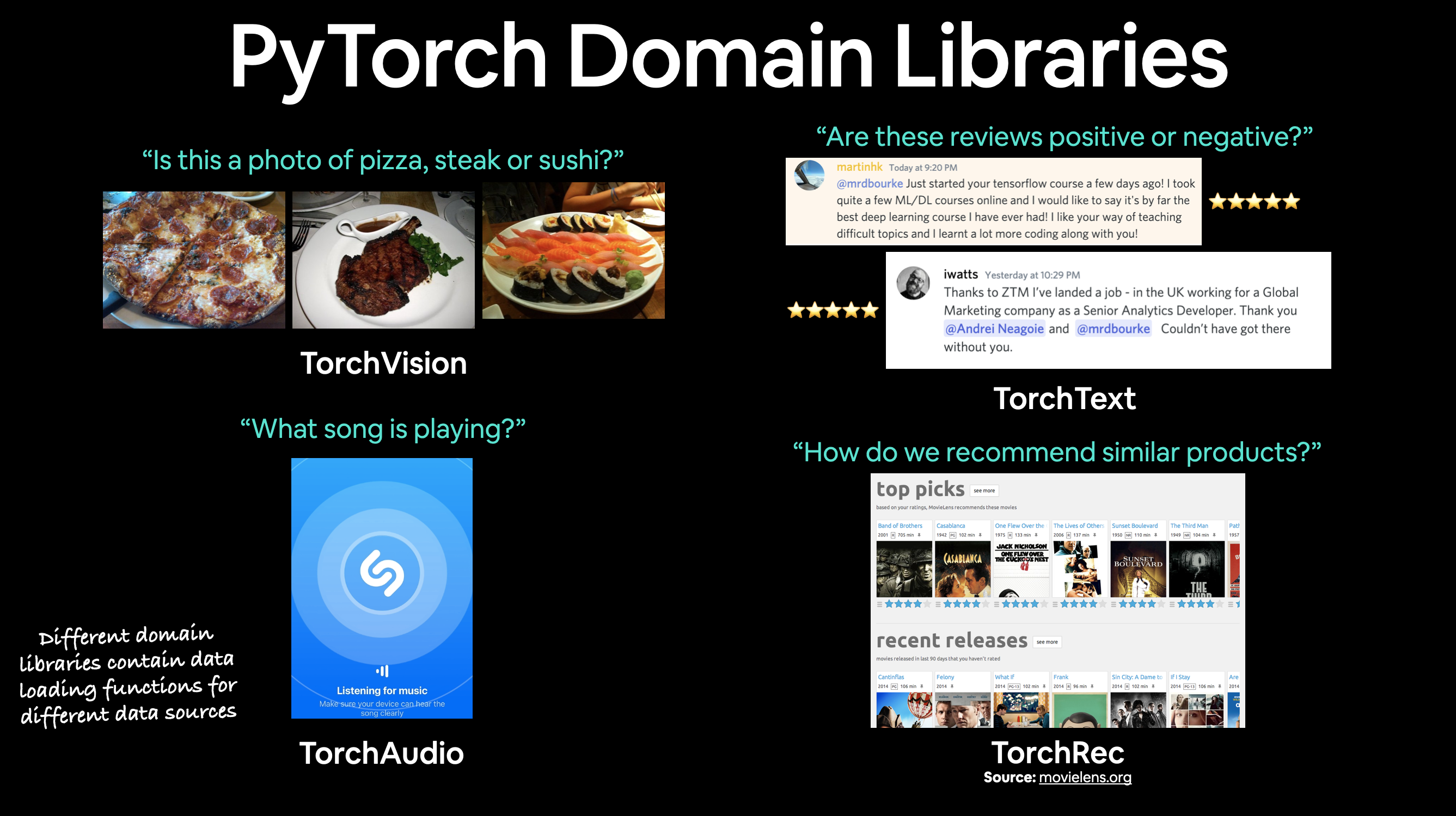
PyTorch에는 TorchVision, TorchText, TorchAudio 및 TorchRec 도메인 라이브러리에 다양한 사용자 정의 데이터셋을 로드하기 위한 많은 기존 함수가 포함되어 있습니다.
하지만 때로는 이러한 기존 함수만으로는 충분하지 않을 수 있습니다.
이러한 경우 항상 torch.utils.data.Dataset을 상속받아 원하는 대로 커스터마이징할 수 있습니다.
노트북 01과 노트북 02에서 다루었던 PyTorch 워크플로우를 컴퓨터 비전 문제에 적용해 보겠습니다.
하지만 PyTorch 내장 데이터셋을 사용하는 대신, 피자, 스테이크, 스시 이미지로 구성된 우리만의 데이터셋을 사용할 것입니다.
목표는 이러한 이미지를 로드한 다음 훈련 및 예측을 위한 모델을 구축하는 것입니다.
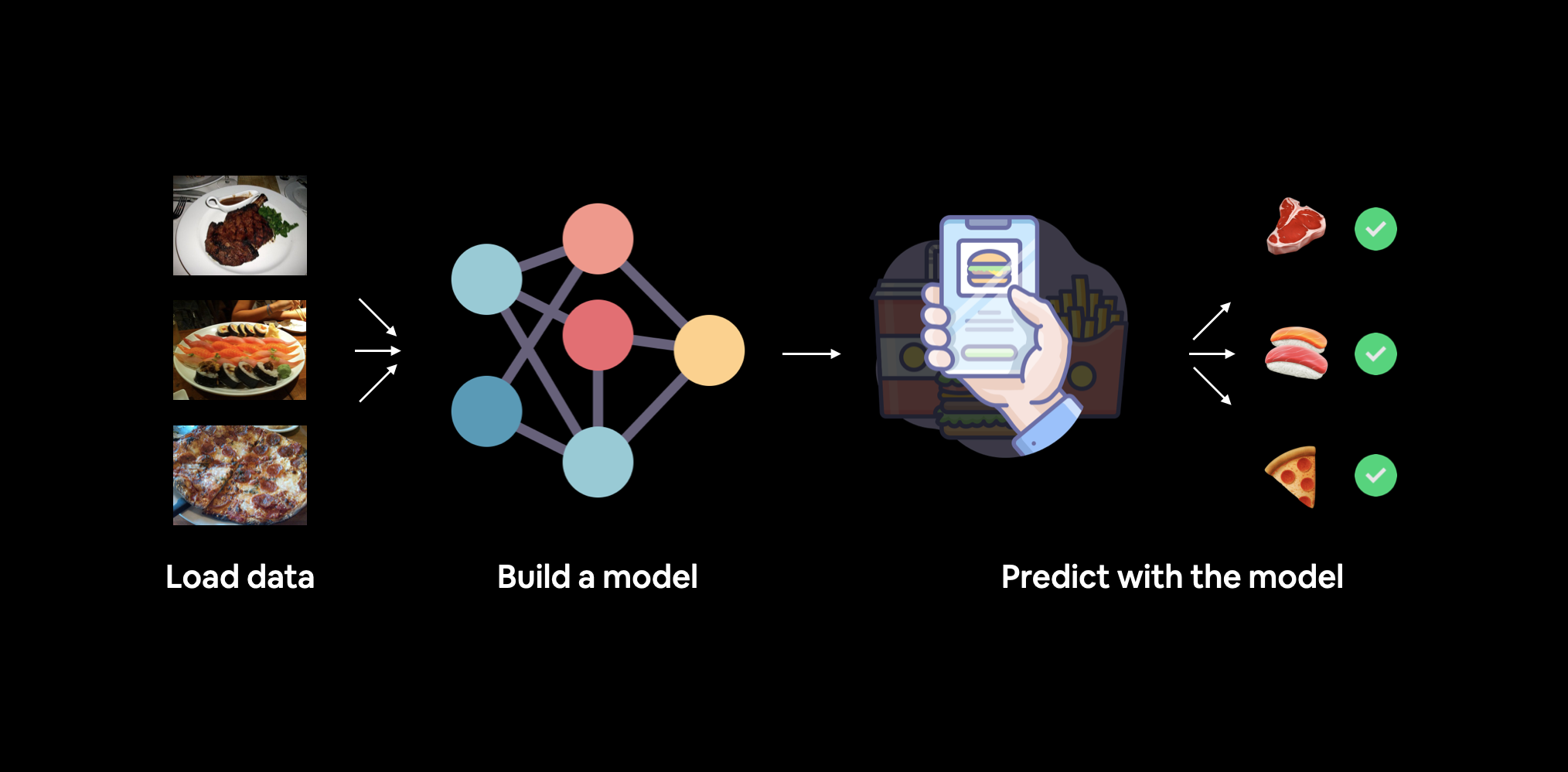
우리가 구축할 내용입니다. torchvision.datasets 뿐만 아니라 자체 사용자 정의 Dataset 클래스를 사용하여 음식 이미지를 로드한 다음, 이를 분류할 수 있는 PyTorch 컴퓨터 비전 모델을 구축할 것입니다.
구체적으로 다음 내용을 다룹니다:
| 주제 | 내용 |
|---|---|
| 0. PyTorch 임포트 및 장치 중립적 코드 설정 | PyTorch를 로드하고 장치 중립적인 코드를 설정하기 위한 권장 사항을 따릅니다. |
| 1. 데이터 가져오기 | 피자, 스테이크, 스시 이미지로 구성된 우리만의 사용자 정의 데이터셋을 사용할 것입니다. |
| 2. 데이터와 하나 되기 (데이터 준비) | 새로운 머신러닝 문제를 시작할 때, 다루고 있는 데이터를 이해하는 것이 가장 중요합니다. 여기서는 우리가 가진 데이터를 파악하기 위한 몇 가지 단계를 거칩니다. |
| 3. 데이터 변환 | 가져온 데이터가 머신러닝 모델에 바로 사용할 수 있는 상태가 아닌 경우가 많습니다. 여기서는 이미지를 모델에 사용할 수 있도록 변환하는 몇 가지 단계를 살펴봅니다. |
4. ImageFolder를 사용하여 데이터 로드 (옵션 1) |
PyTorch에는 일반적인 데이터 유형을 위한 많은 내장 데이터 로딩 함수가 있습니다. ImageFolder는 이미지가 표준 이미지 분류 형식으로 되어 있을 때 유용합니다. |
5. 사용자 정의 Dataset으로 이미지 데이터 로드 |
PyTorch에 내장된 데이터 로딩 함수가 없다면 어떻게 해야 할까요? 여기서 torch.utils.data.Dataset의 자체 사용자 정의 서브클래스를 구축할 수 있습니다. |
| 6. 다른 형태의 변환 (데이터 증강) | 데이터 증강(Data augmentation)은 훈련 데이터의 다양성을 확장하기 위한 일반적인 기술입니다. 여기서는 torchvision의 내장 데이터 증강 함수 중 일부를 살펴봅니다. |
| 7. 모델 0: 데이터 증강이 없는 TinyVGG | 이 단계에서는 데이터가 준비될 것이며, 이를 학습할 수 있는 모델을 구축해 봅니다. 또한 모델을 훈련하고 평가하기 위한 훈련 및 테스트 함수를 만듭니다. |
| 8. 손실 곡선 탐색 | 손실 곡선은 모델이 시간이 지남에 따라 어떻게 훈련/개선되고 있는지 확인하는 좋은 방법입니다. 또한 모델이 과소적합(underfitting) 또는 과적합(overfitting) 상태인지 확인하는 좋은 방법이기도 합니다. |
| 9. 모델 1: 데이터 증강이 있는 TinyVGG | 이제 데이터 증강 없이 모델을 시도해 보았으니, 데이터 증강이 있는 모델을 시도해 보면 어떨까요? |
| 10. 모델 결과 비교 | 서로 다른 모델의 손실 곡선을 비교하여 어떤 모델이 더 성능이 좋은지 확인하고 성능 향상을 위한 몇 가지 옵션에 대해 논의합니다. |
| 11. 사용자 정의 이미지에 대해 예측 수행 | 우리 모델은 피자, 스테이크, 스시 이미지 데이터셋으로 훈련되었습니다. 이 섹션에서는 훈련된 모델을 사용하여 기존 데이터셋 외부의 이미지에 대해 예측하는 방법을 다룹니다. |
이 과정의 모든 자료는 GitHub에 있습니다.
문제가 발생하면 해당 페이지의 Discussions 페이지에서 질문할 수 있습니다.
또한 PyTorch와 관련된 모든 것에 대해 매우 도움이 되는 장소인 PyTorch 문서와 PyTorch 개발자 포럼도 있습니다.
import torch
from torch import nn
# 참고: this notebook requires torch >= 1.10.0
torch.__version__'1.11.0'And now let’s follow best practice and setup device-agnostic code.
참고: If you’re using Google Colab, and you don’t have a GPU turned on yet, it’s now time to turn one on via
Runtime -> Change runtime type -> Hardware accelerator -> GPU. If you do this, your runtime will likely reset and you’ll have to run all of the cells above by goingRuntime -> Run before.
# Setup device-agnostic code
device = "cuda" if torch.cuda.is_available() else "cpu"
device'cuda'First thing’s first we need some data.
And like any good cooking show, some data has already been prepared for us.
We’re going to start small.
Because we’re not looking to train the biggest model or use the biggest dataset yet.
Machine learning is an iterative process, start small, get something working and increase when necessary.
The data we’re going to be using is a subset of the Food101 dataset.
Food101 is popular computer vision benchmark as it contains 1000 images of 101 different kinds of foods, totaling 101,000 images (75,750 train and 25,250 test).
Can you think of 101 different foods?
Can you think of a computer program to classify 101 foods?
I can.
A machine learning model!
Specifically, a PyTorch computer vision model like we covered in notebook 03.
Instead of 101 food classes though, we’re going to start with 3: pizza, steak and sushi.
And instead of 1,000 images per class, we’re going to start with a random 10% (start small, increase when necessary).
If you’d like to see where the data came from you see the following resources: * Original Food101 dataset and paper website. * torchvision.datasets.Food101 - the version of the data I downloaded for this notebook. * extras/04_custom_data_creation.ipynb - a notebook I used to format the Food101 dataset to use for this notebook. * data/pizza_steak_sushi.zip - the zip archive of pizza, steak and sushi images from Food101, created with the notebook linked above.
Let’s write some code to download the formatted data from GitHub.
참고: The dataset we’re about to use has been pre-formatted for what we’d like to use it for. However, you’ll often have to format your own datasets for whatever problem you’re working on. This is a regular practice in the machine learning world.
import requests
import zipfile
from pathlib import Path

# Setup path to data folder
data_path = Path("data/")
image_path = data_path / "pizza_steak_sushi"

# If the image folder doesn't exist, download it and prepare it...
if image_path.is_dir():
    print(f"{image_path} directory exists.")
else:
    print(f"Did not find {image_path} directory, creating one...")
    image_path.mkdir(parents=True, exist_ok=True)

    # Download pizza, steak, sushi data
    with open(data_path / "pizza_steak_sushi.zip", "wb") as f:
        request = requests.get("https://github.com/mrdbourke/pytorch-deep-learning/raw/main/data/pizza_steak_sushi.zip")
        print("Downloading pizza, steak, sushi data...")
        f.write(request.content)

    # Unzip pizza, steak, sushi data
    with zipfile.ZipFile(data_path / "pizza_steak_sushi.zip", "r") as zip_ref:
        print("Unzipping pizza, steak, sushi data...")
        zip_ref.extractall(image_path)
data/pizza_steak_sushi directory exists.Dataset downloaded!
Time to become one with it.
This is another important step before building a model.
As Abraham Lossfunction said…

Data preparation is paramount. Before building a model, become one with the data. Ask: What am I trying to do here? Source: @mrdbourke Twitter.
What’s inspecting the data and becoming one with it?
Before starting a project or building any kind of model, it’s important to know what data you’re working with.
In our case, we have images of pizza, steak and sushi in standard image classification format.
Image classification format contains separate classes of images in seperate directories titled with a particular class name.
For example, all images of pizza are contained in the pizza/ directory.
This format is popular across many different image classification benchmarks, including ImageNet (of the most popular computer vision benchmark datasets).
You can see an example of the storage format below, the images numbers are arbitrary.
pizza_steak_sushi/ <- overall dataset folder
    train/ <- training images
        pizza/ <- class name as folder name
            image01.jpeg
            image02.jpeg
            ...
        steak/
            image24.jpeg
            image25.jpeg
            ...
        sushi/
            image37.jpeg
            ...
    test/ <- testing images
        pizza/
            image101.jpeg
            image102.jpeg
            ...
        steak/
            image154.jpeg
            image155.jpeg
            ...
        sushi/
            image167.jpeg
            ...
The goal will be to take this data storage structure and turn it into a dataset usable with PyTorch.
참고: The structure of the data you work with will vary depending on the problem you’re working on. But the premise still remains: become one with the data, then find a way to best turn it into a dataset compatible with PyTorch.
We can inspect what’s in our data directory by writing a small helper function to walk through each of the subdirectories and count the files present.
To do so, we’ll use Python’s in-built os.walk().
import os
def walk_through_dir(dir_path):
  """
  Walks through dir_path returning its contents.
  Args:
    dir_path (str or pathlib.Path): target directory

  Returns:
    A print out of:
      number of subdiretories in dir_path
      number of images (files) in each subdirectory
      name of each subdirectory
  """
  for dirpath, dirnames, filenames in os.walk(dir_path):
print(f"There are {len(dirnames)} directories and {len(filenames)} images in '{dirpath}'.")walk_through_dir(image_path)There are 2 directories and 0 images in 'data\pizza_steak_sushi'.
There are 3 directories and 0 images in 'data\pizza_steak_sushi\test'.
There are 0 directories and 25 images in 'data\pizza_steak_sushi\test\pizza'.
There are 0 directories and 19 images in 'data\pizza_steak_sushi\test\steak'.
There are 0 directories and 31 images in 'data\pizza_steak_sushi\test\sushi'.
There are 3 directories and 0 images in 'data\pizza_steak_sushi\train'.
There are 0 directories and 78 images in 'data\pizza_steak_sushi\train\pizza'.
There are 0 directories and 75 images in 'data\pizza_steak_sushi\train\steak'.
There are 0 directories and 72 images in 'data\pizza_steak_sushi\train\sushi'.Excellent!
It looks like we’ve got about 75 images per training class and 25 images per testing class.
That should be enough to get started.
Remember, these images are subsets of the original Food101 dataset.
You can see how they were created in the data creation notebook.
While we’re at it, let’s setup our training and testing paths.
# Setup train and testing paths
train_dir = image_path / "train"
test_dir = image_path / "test"

train_dir, test_dir
(WindowsPath('data/pizza_steak_sushi/train'),
WindowsPath('data/pizza_steak_sushi/test'))Okay, we’ve seen how our directory structure is formatted.
Now in the spirit of the data explorer, it’s time to visualize, visualize, visualize!
Let’s write some code to: 1. Get all of the image paths using pathlib.Path.glob() to find all of the files ending in .jpg. 2. Pick a random image path using Python’s random.choice(). 3. Get the image class name using pathlib.Path.parent.stem. 4. And since we’re working with images, we’ll open the random image path using PIL.Image.open() (PIL stands for Python Image Library). 5. We’ll then show the image and print some metadata.
import random
from PIL import Image

# Set seed
random.seed(42) # <- try changing this and see what happens

# 1. Get all image paths (* means "any combination")
image_path_list = list(image_path.glob("*/*/*.jpg"))

# 2. Get random image path
random_image_path = random.choice(image_path_list)

# 3. Get image class from path name (the image class is the name of the directory where the image is stored)
image_class = random_image_path.parent.stem

# 4. Open image
img = Image.open(random_image_path)

# 5. Print metadata
print(f"Random image path: {random_image_path}")
print(f"Image class: {image_class}")
print(f"Image height: {img.height}")
print(f"Image width: {img.width}")
img
Random image path: data\pizza_steak_sushi\test\sushi\2394442.jpg
Image class: sushi
Image height: 408
Image width: 512
We can do the same with matplotlib.pyplot.imshow(), except we have to convert the image to a NumPy array first.
import numpy as np
import matplotlib.pyplot as plt

# Turn the image into an array
img_as_array = np.asarray(img)

# Plot the image with matplotlib
plt.figure(figsize=(10, 7))
plt.imshow(img_as_array)
plt.title(f"Image class: {image_class} | Image shape: {img_as_array.shape} -> [height, width, color_channels]")
plt.axis(False);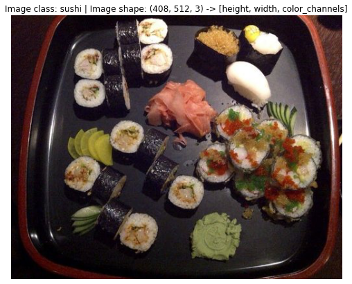
Now what if we wanted to load our image data into PyTorch?
Before we can use our image data with PyTorch we need to:
torch.utils.data.Dataset and subsequently a torch.utils.data.DataLoader, we’ll call these Dataset and DataLoader for short.There are several different kinds of pre-built datasets and dataset loaders for PyTorch, depending on the problem you’re working on.
| Problem space | Pre-built Datasets and Functions |
|---|---|
| Vision | torchvision.datasets |
| Audio | torchaudio.datasets |
| Text | torchtext.datasets |
| Recommendation system | torchrec.datasets |
Since we’re working with a vision problem, we’ll be looking at torchvision.datasets for our data loading functions as well as torchvision.transforms for preparing our data.
Let’s import some base libraries.
import torch
from torch.utils.data import DataLoader
from torchvision import datasets, transformstorchvision.transformsWe’ve got folders of images but before we can use them with PyTorch, we need to convert them into tensors.
One of the ways we can do this is by using the torchvision.transforms module.
torchvision.transforms contains many pre-built methods for formatting images, turning them into tensors and even manipulating them for data augmentation (the practice of altering data to make it harder for a model to learn, we’ll see this later on) purposes .
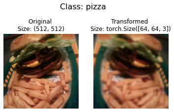
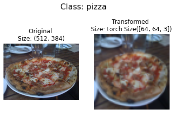
To get experience with torchvision.transforms, let’s write a series of transform steps that: 1. Resize the images using transforms.Resize() (from about 512x512 to 64x64, the same shape as the images on the CNN Explainer website). 2. Flip our images randomly on the horizontal using transforms.RandomHorizontalFlip() (this could be considered a form of data augmentation because it will artificially change our image data). 3. Turn our images from a PIL image to a PyTorch tensor using transforms.ToTensor().
We can compile all of these steps using torchvision.transforms.Compose().
# Write transform for image
data_transform = transforms.Compose([
# Resize the images to 64x64
transforms.Resize(size=(64, 64)),
# Flip the images randomly on the horizontal
transforms.RandomHorizontalFlip(p=0.5), # p = probability of flip, 0.5 = 50% chance
# Turn the image into a torch.Tensor
transforms.ToTensor() # this also converts all pixel values from 0 to 255 to be between 0.0 and 1.0
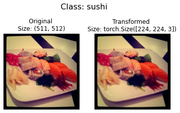
])Now we’ve got a composition of transforms, let’s write a function to try them out on various images.
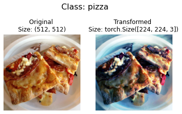
def plot_transformed_images(image_paths, transform, n=3, seed=42):
    """Plots a series of random images from image_paths.

    Will open n image paths from image_paths, transform them
    with transform and plot them side by side.

    Args:
        image_paths (list): List of target image paths.
        transform (PyTorch Transforms): Transforms to apply to images.
        n (int, optional): Number of images to plot. Defaults to 3.
        seed (int, optional): Random seed for the random generator. Defaults to 42.
    """
    random.seed(seed)
    random_image_paths = random.sample(image_paths, k=n)
    for image_path in random_image_paths:
        with Image.open(image_path) as f:
            fig, ax = plt.subplots(1, 2)
            ax[0].imshow(f)
            ax[0].set_title(f"Original \nSize: {f.size}")
            ax[0].axis("off")

            # Transform and plot image
            # 참고: permute() will change shape of image to suit matplotlib
            # (PyTorch default is [C, H, W] but Matplotlib is [H, W, C])
            transformed_image = transform(f).permute(1, 2, 0)
            ax[1].imshow(transformed_image)
            ax[1].set_title(f"Transformed \nSize: {transformed_image.shape}")
            ax[1].axis("off")

            fig.suptitle(f"Class: {image_path.parent.stem}", fontsize=16)

plot_transformed_images(image_path_list,
                        transform=data_transform,
                        n=3)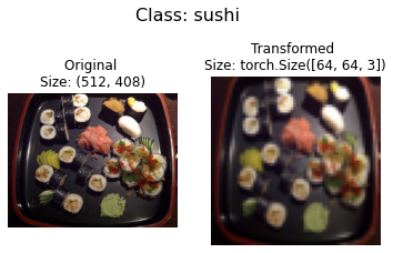
Nice!
We’ve now got a way to convert our images to tensors using torchvision.transforms.
We also manipulate their size and orientation if needed (some models prefer images of different sizes and shapes).
Generally, the larger the shape of the image, the more information a model can recover.
For example, an image of size [256, 256, 3] will have 16x more pixels than an image of size [64, 64, 3] ((256*256*3)/(64*64*3)=16).
However, the tradeoff is that more pixels requires more computations.
Exercise: Try commenting out one of the transforms in
data_transformand running the plotting functionplot_transformed_images()again, what happens?
ImageFolderAlright, time to turn our image data into a Dataset capable of being used with PyTorch.
Since our data is in standard image classification format, we can use the class torchvision.datasets.ImageFolder.
Where we can pass it the file path of a target image directory as well as a series of transforms we’d like to perform on our images.
Let’s test it out on our data folders train_dir and test_dir passing in transform=data_transform to turn our images into tensors.
# Use ImageFolder to create dataset(s)
from torchvision import datasets
train_data = datasets.ImageFolder(root=train_dir, # target folder of images
                                  transform=data_transform, # transforms to perform on data (images)
                                  target_transform=None) # transforms to perform on labels (if necessary)

test_data = datasets.ImageFolder(root=test_dir,
                                 transform=data_transform)

print(f"Train data:\n{train_data}\nTest data:\n{test_data}")
Train data:
Dataset ImageFolder
Number of datapoints: 225
Root location: data\pizza_steak_sushi\train
StandardTransform
Transform: Compose(
Resize(size=(64, 64), interpolation=bilinear, max_size=None, antialias=None)
RandomHorizontalFlip(p=0.5)
ToTensor()
)
Test data:
Dataset ImageFolder
Number of datapoints: 75
Root location: data\pizza_steak_sushi\test
StandardTransform
Transform: Compose(
Resize(size=(64, 64), interpolation=bilinear, max_size=None, antialias=None)
RandomHorizontalFlip(p=0.5)
ToTensor()
)Beautiful!
It looks like PyTorch has registered our Dataset’s.
Let’s inspect them by checking out the classes and class_to_idx attributes as well as the lengths of our training and test sets.
# Get class names as a list
class_names = train_data.classes
class_names
['pizza', 'steak', 'sushi']# Can also get class names as a dict
class_dict = train_data.class_to_idx
class_dict{'pizza': 0, 'steak': 1, 'sushi': 2}# Check the lengths
len(train_data), len(test_data)(225, 75)Nice! Looks like we’ll be able to use these to reference for later.
How about our images and labels?
How do they look?
We can index on our train_data and test_data Dataset’s to find samples and their target labels.
img, label = train_data[0][0], train_data[0][1]
print(f"Image tensor:\n{img}")
print(f"Image shape: {img.shape}")
print(f"Image datatype: {img.dtype}")
print(f"Image label: {label}")
print(f"Label datatype: {type(label)}")
Image tensor:
tensor([[[0.1137, 0.1020, 0.0980, ..., 0.1255, 0.1216, 0.1176],
[0.1059, 0.0980, 0.0980, ..., 0.1294, 0.1294, 0.1294],
[0.1020, 0.0980, 0.0941, ..., 0.1333, 0.1333, 0.1333],
...,
[0.1098, 0.1098, 0.1255, ..., 0.1686, 0.1647, 0.1686],
[0.0863, 0.0941, 0.1098, ..., 0.1686, 0.1647, 0.1686],
[0.0863, 0.0863, 0.0980, ..., 0.1686, 0.1647, 0.1647]],
[[0.0745, 0.0706, 0.0745, ..., 0.0588, 0.0588, 0.0588],
[0.0706, 0.0706, 0.0745, ..., 0.0627, 0.0627, 0.0627],
[0.0706, 0.0745, 0.0745, ..., 0.0706, 0.0706, 0.0706],
...,
[0.1255, 0.1333, 0.1373, ..., 0.2510, 0.2392, 0.2392],
[0.1098, 0.1176, 0.1255, ..., 0.2510, 0.2392, 0.2314],
[0.1020, 0.1059, 0.1137, ..., 0.2431, 0.2353, 0.2275]],
[[0.0941, 0.0902, 0.0902, ..., 0.0196, 0.0196, 0.0196],
[0.0902, 0.0863, 0.0902, ..., 0.0196, 0.0157, 0.0196],
[0.0902, 0.0902, 0.0902, ..., 0.0157, 0.0157, 0.0196],
...,
[0.1294, 0.1333, 0.1490, ..., 0.1961, 0.1882, 0.1804],
[0.1098, 0.1137, 0.1255, ..., 0.1922, 0.1843, 0.1804],
[0.1059, 0.1020, 0.1059, ..., 0.1843, 0.1804, 0.1765]]])
Image shape: torch.Size([3, 64, 64])
Image datatype: torch.float32
Image label: 0
Label datatype: <class 'int'>Our images are now in the form of a tensor (with shape [3, 64, 64]) and the labels are in the form of an integer relating to a specific class (as referenced by the class_to_idx attribute).
How about we plot a single image tensor using matplotlib?
We’ll first have to to permute (rearrange the order of its dimensions) so it’s compatible.
Right now our image dimensions are in the format CHW (color channels, height, width) but matplotlib prefers HWC (height, width, color channels).
# Rearrange the order of dimensions
img_permute = img.permute(1, 2, 0)

# Print out different shapes (before and after permute)
print(f"Original shape: {img.shape} -> [color_channels, height, width]")
print(f"Image permute shape: {img_permute.shape} -> [height, width, color_channels]")

# Plot the image
plt.figure(figsize=(10, 7))
plt.imshow(img.permute(1, 2, 0))
plt.axis("off")
plt.title(class_names[label], fontsize=14);
Original shape: torch.Size([3, 64, 64]) -> [color_channels, height, width]
Image permute shape: torch.Size([64, 64, 3]) -> [height, width, color_channels]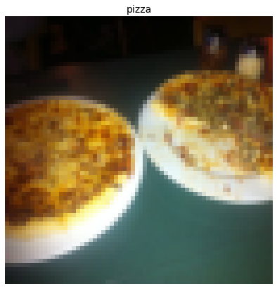
Notice the image is now more pixelated (less quality).
This is due to it being resized from 512x512 to 64x64 pixels.
The intuition here is that if you think the image is harder to recognize what’s going on, chances are a model will find it harder to understand too.
DataLoader’sWe’ve got our images as PyTorch Dataset’s but now let’s turn them into DataLoader’s.
We’ll do so using torch.utils.data.DataLoader.
Turning our Dataset’s into DataLoader’s makes them iterable so a model can go through learn the relationships between samples and targets (features and labels).
To keep things simple, we’ll use a batch_size=1 and num_workers=1.
What’s num_workers?
Good question.
It defines how many subprocesses will be created to load your data.
Think of it like this, the higher value num_workers is set to, the more compute power PyTorch will use to load your data.
Personally, I usually set it to the total number of CPUs on my machine via Python’s os.cpu_count().
This ensures the DataLoader recruits as many cores as possible to load data.
참고: There are more parameters you can get familiar with using
torch.utils.data.DataLoaderin the PyTorch documentation.
# Turn train and test Datasets into DataLoaders
from torch.utils.data import DataLoader
train_dataloader = DataLoader(dataset=train_data,
                              batch_size=1, # how many samples per batch?
                              num_workers=1, # how many subprocesses to use for data loading? (higher = more)
                              shuffle=True) # shuffle the data?

test_dataloader = DataLoader(dataset=test_data,
                             batch_size=1,
                             num_workers=1,
                             shuffle=False) # don't usually need to shuffle testing data

train_dataloader, test_dataloader
(<torch.utils.data.dataloader.DataLoader at 0x1fd2cf94fa0>,
<torch.utils.data.dataloader.DataLoader at 0x1fd2cf94dc0>)Wonderful!
Now our data is iterable.
Let’s try it out and check the shapes.
img, label = next(iter(train_dataloader))

# Batch size will now be 1, try changing the batch_size parameter above and see what happens
print(f"Image shape: {img.shape} -> [batch_size, color_channels, height, width]")
print(f"Label shape: {label.shape}")
Image shape: torch.Size([1, 3, 64, 64]) -> [batch_size, color_channels, height, width]
Label shape: torch.Size([1])We could now use these DataLoader’s with a training and testing loop to train a model.
But before we do, let’s look at another option to load images (or almost any other kind of data).
DatasetWhat if a pre-built Dataset creator like torchvision.datasets.ImageFolder() didn’t exist?
Or one for your specific problem didn’t exist?
Well, you could build your own.
But wait, what are the pros and cons of creating your own custom way to load Dataset’s?
Pros of creating a custom Dataset |
Cons of creating a custom Dataset |
|---|---|
Can create a Dataset out of almost anything. |
Even though you could create a Dataset out of almost anything, it doesn’t mean it will work. |
Not limited to PyTorch pre-built Dataset functions. |
Using a custom Dataset often results in writing more code, which could be prone to errors or performance issues. |
To see this in action, let’s work towards replicating torchvision.datasets.ImageFolder() by subclassing torch.utils.data.Dataset (the base class for all Dataset’s in PyTorch).
We’ll start by importing the modules we need: * Python’s os for dealing with directories (our data is stored in directories). * Python’s pathlib for dealing with filepaths (each of our images has a unique filepath). * torch for all things PyTorch. * PIL’s Image class for loading images. * torch.utils.data.Dataset to subclass and create our own custom Dataset. * torchvision.transforms to turn our images into tensors. * Various types from Python’s typing module to add type hints to our code.
참고: You can customize the following steps for your own dataset. The premise remains: write code to load your data in the format you’d like it.
import os
import pathlib
import torch

from PIL import Image
from torch.utils.data import Dataset
from torchvision import transforms
from typing import Tuple, Dict, List
Remember how our instances of torchvision.datasets.ImageFolder() allowed us to use the classes and class_to_idx attributes?
# Instance of torchvision.datasets.ImageFolder()
train_data.classes, train_data.class_to_idx
(['pizza', 'steak', 'sushi'], {'pizza': 0, 'steak': 1, 'sushi': 2})Let’s write a helper function capable of creating a list of class names and a dictionary of class names and their indexes given a directory path.
To do so, we’ll: 1. Get the class names using os.scandir() to traverse a target directory (ideally the directory is in standard image classification format). 2. Raise an error if the class names aren’t found (if this happens, there might be something wrong with the directory structure). 3. Turn the class names into a dictionary of numerical labels, one for each class.
Let’s see a small example of step 1 before we write the full function.
# Setup path for target directory
target_directory = train_dir
print(f"Target directory: {target_directory}")

# Get the class names from the target directory
class_names_found = sorted([entry.name for entry in list(os.scandir(image_path / "train"))])
print(f"Class names found: {class_names_found}")
Target directory: data\pizza_steak_sushi\train
Class names found: ['pizza', 'steak', 'sushi']Excellent!
How about we turn it into a full function?
# Make function to find classes in target directory
def find_classes(directory: str) -> Tuple[List[str], Dict[str, int]]:
    """Finds the class folder names in a target directory.

    Assumes target directory is in standard image classification format.

    Args:
        directory (str): target directory to load classnames from.

    Returns:
        Tuple[List[str], Dict[str, int]]: (list_of_class_names, dict(class_name: idx...))

    Example:
        find_classes("food_images/train")
        >>> (["class_1", "class_2"], {"class_1": 0, ...})
    """
    # 1. Get the class names by scanning the target directory
    classes = sorted(entry.name for entry in os.scandir(directory) if entry.is_dir())

    # 2. Raise an error if class names not found
    if not classes:
        raise FileNotFoundError(f"Couldn't find any classes in {directory}.")

    # 3. Crearte a dictionary of index labels (computers prefer numerical rather than string labels)
    class_to_idx = {cls_name: i for i, cls_name in enumerate(classes)}
    return classes, class_to_idx
Looking good!
Now let’s test out our find_classes() function.
find_classes(train_dir)(['pizza', 'steak', 'sushi'], {'pizza': 0, 'steak': 1, 'sushi': 2})Woohoo! Looking good!
Dataset to replicate ImageFolderNow we’re ready to build our own custom Dataset.
We’ll build one to replicate the functionality of torchvision.datasets.ImageFolder().
This will be good practice, plus, it’ll reveal a few of the required steps to make your own custom Dataset.
It’ll be a fair bit of a code… but nothing we can’t handle!
Let’s break it down: 1. Subclass torch.utils.data.Dataset. 2. Initialize our subclass with a targ_dir parameter (the target data directory) and transform parameter (so we have the option to transform our data if needed). 3. Create several attributes for paths (the paths of our target images), transform (the transforms we might like to use, this can be None), classes and class_to_idx (from our find_classes() function). 4. Create a function to load images from file and return them, this could be using PIL or torchvision.io (for input/output of vision data). 5. Overwrite the __len__ method of torch.utils.data.Dataset to return the number of samples in the Dataset, this is recommended but not required. This is so you can call len(Dataset). 6. Overwrite the __getitem__ method of torch.utils.data.Dataset to return a single sample from the Dataset, this is required.
Let’s do it!
# Write a custom dataset class (inherits from torch.utils.data.Dataset)
from torch.utils.data import Dataset

# 1. Subclass torch.utils.data.Dataset
class ImageFolderCustom(Dataset):

    # 2. Initialize with a targ_dir and transform (optional) parameter
    def __init__(self, targ_dir: str, transform=None) -> None:

        # 3. Create class attributes
        # Get all image paths
        self.paths = list(pathlib.Path(targ_dir).glob("*/*.jpg")) # note: you'd have to update this if you've got .png's or .jpeg's
        # Setup transforms
        self.transform = transform
        # Create classes and class_to_idx attributes
        self.classes, self.class_to_idx = find_classes(targ_dir)

    # 4. Make function to load images
    def load_image(self, index: int) -> Image.Image:
        "Opens an image via a path and returns it."
        image_path = self.paths[index]
        return Image.open(image_path)

    # 5. Overwrite the __len__() method (optional but recommended for subclasses of torch.utils.data.Dataset)
    def __len__(self) -> int:
        "Returns the total number of samples."
        return len(self.paths)

    # 6. Overwrite the __getitem__() method (required for subclasses of torch.utils.data.Dataset)
    def __getitem__(self, index: int) -> Tuple[torch.Tensor, int]:
        "Returns one sample of data, data and label (X, y)."
        img = self.load_image(index)
        class_name  = self.paths[index].parent.name # expects path in data_folder/class_name/image.jpeg
        class_idx = self.class_to_idx[class_name]

        # Transform if necessary
        if self.transform:
            return self.transform(img), class_idx # return data, label (X, y)
        else:
            return img, class_idx # return data, label (X, y)
Woah! A whole bunch of code to load in our images.
This is one of the downsides of creating your own custom Dataset’s.
However, now we’ve written it once, we could move it into a .py file such as data_loader.py along with some other helpful data functions and reuse it later on.
Before we test out our new ImageFolderCustom class, let’s create some transforms to prepare our images.
# Augment train data
train_transforms = transforms.Compose([
    transforms.Resize((64, 64)),
    transforms.RandomHorizontalFlip(p=0.5),
    transforms.ToTensor()
])

# Don't augment test data, only reshape
test_transforms = transforms.Compose([
    transforms.Resize((64, 64)),
    transforms.ToTensor()
])
Now comes the moment of truth!
Let’s turn our training images (contained in train_dir) and our testing images (contained in test_dir) into Dataset’s using our own ImageFolderCustom class.
train_data_custom = ImageFolderCustom(targ_dir=train_dir,
                                      transform=train_transforms)
test_data_custom = ImageFolderCustom(targ_dir=test_dir,
                                     transform=test_transforms)
train_data_custom, test_data_custom
(<__main__.ImageFolderCustom at 0x1fd2cf886d0>,
<__main__.ImageFolderCustom at 0x1fd2cf5a0d0>)Hmm… no errors, did it work?
Let’s try calling len() on our new Dataset’s and find the classes and class_to_idx attributes.
len(train_data_custom), len(test_data_custom)(225, 75)train_data_custom.classes['pizza', 'steak', 'sushi']train_data_custom.class_to_idx{'pizza': 0, 'steak': 1, 'sushi': 2}len(test_data_custom) == len(test_data) and len(test_data_custom) == len(test_data) Yes!!!
It looks like it worked.
We could check for equality with the Dataset’s made by the torchvision.datasets.ImageFolder() class too.
# Check for equality amongst our custom Dataset and ImageFolder Dataset
print((len(train_data_custom) == len(train_data)) & (len(test_data_custom) == len(test_data)))
print(train_data_custom.classes == train_data.classes)
print(train_data_custom.class_to_idx == train_data.class_to_idx)
True
True
TrueHo ho!
Look at us go!
Three True’s!
You can’t get much better than that.
How about we take it up a notch and plot some random images to test our __getitem__ override?
You know what time it is!
Time to put on our data explorer’s hat and visualize, visualize, visualize!
Let’s create a helper function called display_random_images() that helps us visualize images in our Dataset's.
Specifically, it’ll: 1. Take in a Dataset and a number of other parameters such as classes (the names of our target classes), the number of images to display (n) and a random seed. 2. To prevent the display getting out of hand, we’ll cap n at 10 images. 3. Set the random seed for reproducible plots (if seed is set). 4. Get a list of random sample indexes (we can use Python’s random.sample() for this) to plot. 5. Setup a matplotlib plot. 6. Loop through the random sample indexes found in step 4 and plot them with matplotlib. 7. Make sure the sample images are of shape HWC (height, width, color channels) so we can plot them.
# 1. Take in a Dataset as well as a list of class names
def display_random_images(dataset: torch.utils.data.dataset.Dataset,
                          classes: List[str] = None,
                          n: int = 10,
                          display_shape: bool = True,
                          seed: int = None):

    # 2. Adjust display if n too high
    if n > 10:
        n = 10
        display_shape = False
        print(f"For display purposes, n shouldn't be larger than 10, setting to 10 and removing shape display.")

    # 3. Set random seed
    if seed:
        random.seed(seed)

    # 4. Get random sample indexes
    random_samples_idx = random.sample(range(len(dataset)), k=n)

    # 5. Setup plot
    plt.figure(figsize=(16, 8))

    # 6. Loop through samples and display random samples
    for i, targ_sample in enumerate(random_samples_idx):
        targ_image, targ_label = dataset[targ_sample][0], dataset[targ_sample][1]

        # 7. Adjust image tensor shape for plotting: [color_channels, height, width] -> [color_channels, height, width]
        targ_image_adjust = targ_image.permute(1, 2, 0)

        # Plot adjusted samples
        plt.subplot(1, n, i+1)
        plt.imshow(targ_image_adjust)
        plt.axis("off")
        if classes:
            title = f"class: {classes[targ_label]}"
            if display_shape:
                title = title + f"\nshape: {targ_image_adjust.shape}"
        plt.title(title)
What a good looking function!
Let’s test it out first with the Dataset we created with torchvision.datasets.ImageFolder().
# Display random images from ImageFolder created Dataset
display_random_images(train_data,
                      n=5,
                      classes=class_names,
                      seed=None)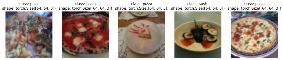
And now with the Dataset we created with our own ImageFolderCustom.
# Display random images from ImageFolderCustom Dataset
display_random_images(train_data_custom,
                      n=12,
                      classes=class_names,
                      seed=None) # Try setting the seed for reproducible images
For display purposes, n shouldn't be larger than 10, setting to 10 and removing shape display.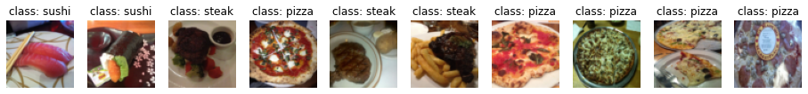
Nice!!!
Looks like our ImageFolderCustom is working just as we’d like it to.
DataLoader’sWe’ve got a way to turn our raw images into Dataset’s (features mapped to labels or X’s mapped to y’s) through our ImageFolderCustom class.
Now how could we turn our custom Dataset’s into DataLoader’s?
If you guessed by using torch.utils.data.DataLoader(), you’d be right!
Because our custom Dataset’s subclass torch.utils.data.Dataset, we can use them directly with torch.utils.data.DataLoader().
And we can do using very similar steps to before except this time we’ll be using our custom created Dataset’s.
# Turn train and test custom Dataset's into DataLoader's
from torch.utils.data import DataLoader
train_dataloader_custom = DataLoader(dataset=train_data_custom, # use custom created train Dataset
                                     batch_size=1, # how many samples per batch?
                                     num_workers=0, # how many subprocesses to use for data loading? (higher = more)
                                     shuffle=True) # shuffle the data?

test_dataloader_custom = DataLoader(dataset=test_data_custom, # use custom created test Dataset
                                    batch_size=1,
                                    num_workers=0,
                                    shuffle=False) # don't usually need to shuffle testing data

train_dataloader_custom, test_dataloader_custom
(<torch.utils.data.dataloader.DataLoader at 0x1fd2cfabf10>,
<torch.utils.data.dataloader.DataLoader at 0x1fd2cfabb80>)Do the shapes of the samples look the same?
# Get image and label from custom DataLoader
img_custom, label_custom = next(iter(train_dataloader_custom))

# Batch size will now be 1, try changing the batch_size parameter above and see what happens
print(f"Image shape: {img_custom.shape} -> [batch_size, color_channels, height, width]")
print(f"Label shape: {label_custom.shape}")
Image shape: torch.Size([1, 3, 64, 64]) -> [batch_size, color_channels, height, width]
Label shape: torch.Size([1])They sure do!
Let’s now take a lot at some other forms of data transforms.
We’ve seen a couple of transforms on our data already but there’s plenty more.
You can see them all in the torchvision.transforms documentation.
The purpose of tranforms is to alter your images in some way.
That may be turning your images into a tensor (as we’ve seen before).
Or cropping it or randomly erasing a portion or randomly rotating them.
Doing this kinds of transforms is often referred to as data augmentation.
Data augmentation is the process of altering your data in such a way that you artificially increase the diversity of your training set.
Training a model on this artificially altered dataset hopefully results in a model that is capable of better generalization (the patterns it learns are more robust to future unseen examples).
You can see many different examples of data augmentation performed on images using torchvision.transforms in PyTorch’s Illustration of Transforms example.
But let’s try one out ourselves.
Machine learning is all about harnessing the power of randomness and research shows that random transforms (like transforms.RandAugment() and transforms.TrivialAugmentWide()) generally perform better than hand-picked transforms.
The idea behind TrivialAugment is… well, trivial.
You have a set of transforms and you randomly pick a number of them to perform on an image and at a random magnitude between a given range (a higher magnitude means more instense).
The PyTorch team even used TrivialAugment it to train their latest state-of-the-art vision models.
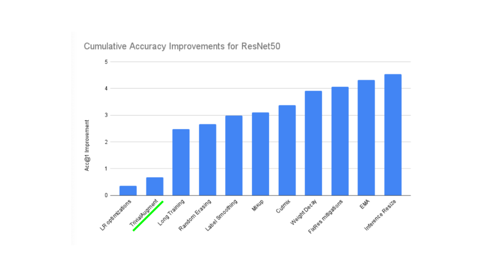
TrivialAugment was one of the ingredients used in a recent state of the art training upgrade to various PyTorch vision models.
How about we test it out on some of our own images?
The main parameter to pay attention to in transforms.TrivialAugmentWide() is num_magnitude_bins=31.
It defines how much of a range an intensity value will be picked to apply a certain transform, 0 being no range and 31 being maximum range (highest chance for highest intensity).
We can incorporate transforms.TrivialAugmentWide() into transforms.Compose().
from torchvision import transforms

train_transforms = transforms.Compose([
    transforms.Resize((224, 224)),
    transforms.TrivialAugmentWide(num_magnitude_bins=31), # how intense
    transforms.ToTensor() # use ToTensor() last to get everything between 0 & 1
])

# Don't need to perform augmentation on the test data
test_transforms = transforms.Compose([
    transforms.Resize((224, 224)),
    transforms.ToTensor()
])
참고: You usually don’t perform data augmentation on the test set. The idea of data augmentation is to to artificially increase the diversity of the training set to better predict on the testing set.
However, you do need to make sure your test set images are transformed to tensors. We size the test images to the same size as our training images too, however, inference can be done on different size images if necessary (though this may alter performance).
Beautiful, now we’ve got a training transform (with data augmentation) and test transform (without data augmentation).
Let’s test our data augmentation out!
# Get all image paths
image_path_list = list(image_path.glob("*/*/*.jpg"))

# Plot random images
plot_transformed_images(
    image_paths=image_path_list,
    transform=train_transforms,
    n=3,
    seed=None
)
Try running the cell above a few times and seeing how the original image changes as it goes through the transform.
Alright, we’ve seen how to turn our data from images in folders to transformed tensors.
Now let’s construct a computer vision model to see if we can classify if an image is of pizza, steak or sushi.
To begin, we’ll start with a simple transform, only resizing the images to (64, 64) and turning them into tensors.
# Create simple transform
simple_transform = transforms.Compose([
    transforms.Resize((64, 64)),
    transforms.ToTensor(),
])
Excellent, now we’ve got a simple transform, let’s: 1. Load the data, turning each of our training and test folders first into a Dataset with torchvision.datasets.ImageFolder() 2. Then into a DataLoader using torch.utils.data.DataLoader(). * We’ll set the batch_size=32 and num_workers to as many CPUs on our machine (this will depend on what machine you’re using).
# 1. Load and transform data
from torchvision import datasets
train_data_simple = datasets.ImageFolder(root=train_dir, transform=simple_transform)
test_data_simple = datasets.ImageFolder(root=test_dir, transform=simple_transform)

# 2. Turn data into DataLoaders
import os
from torch.utils.data import DataLoader

# Setup batch size and number of workers
BATCH_SIZE = 32
NUM_WORKERS = os.cpu_count()
print(f"Creating DataLoader's with batch size {BATCH_SIZE} and {NUM_WORKERS} workers.")

# Create DataLoader's
train_dataloader_simple = DataLoader(train_data_simple,
                                     batch_size=BATCH_SIZE,
                                     shuffle=True,
                                     num_workers=NUM_WORKERS)

test_dataloader_simple = DataLoader(test_data_simple,
                                    batch_size=BATCH_SIZE,
                                    shuffle=False,
                                    num_workers=NUM_WORKERS)

train_dataloader_simple, test_dataloader_simple
Creating DataLoader's with batch size 32 and 16 workers.(<torch.utils.data.dataloader.DataLoader at 0x1fd2ce5c4f0>,
<torch.utils.data.dataloader.DataLoader at 0x1fd1d0e10d0>)DataLoader’s created!
Let’s build a model.
In notebook 03, we used the TinyVGG model from the CNN Explainer website.
Let’s recreate the same model, except this time we’ll be using color images instead of grayscale (in_channels=3 instead of in_channels=1 for RGB pixels).
class TinyVGG(nn.Module):
    """
    Model architecture copying TinyVGG from:
    https://poloclub.github.io/cnn-explainer/
    """
    def __init__(self, input_shape: int, hidden_units: int, output_shape: int) -> None:
        super().__init__()
        self.conv_block_1 = nn.Sequential(
            nn.Conv2d(in_channels=input_shape,
                      out_channels=hidden_units,
                      kernel_size=3, # how big is the square that's going over the image?
                      stride=1, # default
                      padding=1), # options = "valid" (no padding) or "same" (output has same shape as input) or int for specific number
            nn.ReLU(),
            nn.Conv2d(in_channels=hidden_units,
                      out_channels=hidden_units,
                      kernel_size=3,
                      stride=1,
                      padding=1),
            nn.ReLU(),
            nn.MaxPool2d(kernel_size=2,
                         stride=2) # default stride value is same as kernel_size
        )
        self.conv_block_2 = nn.Sequential(
            nn.Conv2d(hidden_units, hidden_units, kernel_size=3, padding=1),
            nn.ReLU(),
            nn.Conv2d(hidden_units, hidden_units, kernel_size=3, padding=1),
            nn.ReLU(),
            nn.MaxPool2d(2)
        )
        self.classifier = nn.Sequential(
            nn.Flatten(),
            # Where did this in_features shape come from?
            # It's because each layer of our network compresses and changes the shape of our inputs data.
            nn.Linear(in_features=hidden_units*16*16,
                      out_features=output_shape)
        )

    def forward(self, x: torch.Tensor):
        x = self.conv_block_1(x)
        # print(x.shape)
        x = self.conv_block_2(x)
        # print(x.shape)
        x = self.classifier(x)
        # print(x.shape)
        return x
        # return self.classifier(self.conv_block_2(self.conv_block_1(x))) # <- leverage the benefits of operator fusion

torch.manual_seed(42)
model_0 = TinyVGG(input_shape=3, # number of color channels (3 for RGB)
                  hidden_units=10,
                  output_shape=len(train_data.classes)).to(device)
model_0
TinyVGG(
(conv_block_1): Sequential(
(0): Conv2d(3, 10, kernel_size=(3, 3), stride=(1, 1), padding=(1, 1))
(1): ReLU()
(2): Conv2d(10, 10, kernel_size=(3, 3), stride=(1, 1), padding=(1, 1))
(3): ReLU()
(4): MaxPool2d(kernel_size=2, stride=2, padding=0, dilation=1, ceil_mode=False)
)
(conv_block_2): Sequential(
(0): Conv2d(10, 10, kernel_size=(3, 3), stride=(1, 1), padding=(1, 1))
(1): ReLU()
(2): Conv2d(10, 10, kernel_size=(3, 3), stride=(1, 1), padding=(1, 1))
(3): ReLU()
(4): MaxPool2d(kernel_size=2, stride=2, padding=0, dilation=1, ceil_mode=False)
)
(classifier): Sequential(
(0): Flatten(start_dim=1, end_dim=-1)
(1): Linear(in_features=2560, out_features=3, bias=True)
)
)참고: One of the ways to speed up deep learning models computing on a GPU is to leverage operator fusion.
This means in the
forward()method in our model above, instead of calling a layer block and reassigningxevery time, we call each block in succession (see the final line of theforward()method in the model above for an example).This saves the time spent reassigning
x(memory heavy) and focuses on only computing onx.See Making Deep Learning Go Brrrr From First Principles by Horace He for more ways on how to speed up machine learning models.
Now that’s a nice looking model!
How about we test it out with a forward pass on a single image?
A good way to test a model is to do a forward pass on a single piece of data.
It’s also handy way to test the input and output shapes of our different layers.
To do a forward pass on a single image, let’s: 1. Get a batch of images and labels from the DataLoader. 2. Get a single image from the batch and unsqueeze() the image so it has a batch size of 1 (so its shape fits the model). 3. Perform inference on a single image (making sure to send the image to the target device). 4. Print out what’s happening and convert the model’s raw output logits to prediction probabilities with torch.softmax() (since we’re working with multi-class data) and convert the prediction probabilities to prediction labels with torch.argmax().
# 1. Get a batch of images and labels from the DataLoader
img_batch, label_batch = next(iter(train_dataloader_simple))

# 2. Get a single image from the batch and unsqueeze the image so its shape fits the model
img_single, label_single = img_batch[0].unsqueeze(dim=0), label_batch[0]
print(f"Single image shape: {img_single.shape}\n")

# 3. Perform a forward pass on a single image
model_0.eval()
with torch.inference_mode():
    pred = model_0(img_single.to(device))

# 4. Print out what's happening and convert model logits -> pred probs -> pred label
print(f"Output logits:\n{pred}\n")
print(f"Output prediction probabilities:\n{torch.softmax(pred, dim=1)}\n")
print(f"Output prediction label:\n{torch.argmax(torch.softmax(pred, dim=1), dim=1)}\n")
print(f"Actual label:\n{label_single}")
Single image shape: torch.Size([1, 3, 64, 64])
Output logits:
tensor([[0.0578, 0.0635, 0.0352]], device='cuda:0')
Output prediction probabilities:
tensor([[0.3352, 0.3371, 0.3277]], device='cuda:0')
Output prediction label:
tensor([1], device='cuda:0')
Actual label:
2Wonderful, it looks like our model is outputting what we’d expect it to output.
You can run the cell above a few times and each time have a different image be predicted on.
And you’ll probably notice the predictions are often wrong.
This is to be expected because the model hasn’t been trained yet and it’s essentially guessing using random weights.
torchinfo to get an idea of the shapes going through our modelPrinting out our model with print(model) gives us an idea of what’s going on with our model.
And we can print out the shapes of our data throughout the forward() method.
However, a helpful way to get information from our model is to use torchinfo.
torchinfo comes with a summary() method that takes a PyTorch model as well as an input_shape and returns what happens as a tensor moves through your model.
참고: If you’re using Google Colab, you’ll need to install
torchinfo.
# Install torchinfo if it's not available, import it if it is
try:
    import torchinfo
except:
    !pip install torchinfo
    import torchinfo

from torchinfo import summary
summary(model_0, input_size=[1, 3, 64, 64]) # do a test pass through of an example input size
Collecting torchinfo
Downloading torchinfo-1.6.5-py3-none-any.whl (21 kB)
Installing collected packages: torchinfo
Successfully installed torchinfo-1.6.5==========================================================================================
Layer (type:depth-idx) Output Shape Param #
==========================================================================================
TinyVGG -- --
├─Sequential: 1-1 [1, 10, 32, 32] --
│ └─Conv2d: 2-1 [1, 10, 64, 64] 280
│ └─ReLU: 2-2 [1, 10, 64, 64] --
│ └─Conv2d: 2-3 [1, 10, 64, 64] 910
│ └─ReLU: 2-4 [1, 10, 64, 64] --
│ └─MaxPool2d: 2-5 [1, 10, 32, 32] --
├─Sequential: 1-2 [1, 10, 16, 16] --
│ └─Conv2d: 2-6 [1, 10, 32, 32] 910
│ └─ReLU: 2-7 [1, 10, 32, 32] --
│ └─Conv2d: 2-8 [1, 10, 32, 32] 910
│ └─ReLU: 2-9 [1, 10, 32, 32] --
│ └─MaxPool2d: 2-10 [1, 10, 16, 16] --
├─Sequential: 1-3 [1, 3] --
│ └─Flatten: 2-11 [1, 2560] --
│ └─Linear: 2-12 [1, 3] 7,683
==========================================================================================
Total params: 10,693
Trainable params: 10,693
Non-trainable params: 0
Total mult-adds (M): 6.75
==========================================================================================
Input size (MB): 0.05
Forward/backward pass size (MB): 0.82
Params size (MB): 0.04
Estimated Total Size (MB): 0.91
==========================================================================================Nice!
The output of torchinfo.summary() gives us a whole bunch of information about our model.
Such as Total params, the total number of parameters in our model, the Estimated Total Size (MB) which is the size of our model.
You can also see the change in input and output shapes as data of a certain input_size moves through our model.
Right now, our parameter numbers and total model size is low.
This because we’re starting with a small model.
And if we need to increase its size later, we can.
We’ve got data and we’ve got a model.
Now let’s make some training and test loop functions to train our model on the training data and evaluate our model on the testing data.
And to make sure we can use these the training and testing loops again, we’ll functionize them.
Specifically, we’re going to make three functions: 1. train_step() - takes in a model, a DataLoader, a loss function and an optimizer and trains the model on the DataLoader. 2. test_step() - takes in a model, a DataLoader and a loss function and evaluates the model on the DataLoader. 3. train() - performs 1. and 2. together for a given number of epochs and returns a results dictionary.
참고: We covered the steps in a PyTorch opimization loop in notebook 01, as well as theUnofficial PyTorch Optimization Loop Song and we’ve built similar functions in notebook 03.
Let’s start by building train_step().
Because we’re dealing with batches in the DataLoader’s, we’ll accumulate the model loss and accuracy values during training (by adding them up for each batch) and then adjust them at the end before we return them.
def train_step(model: torch.nn.Module,
               dataloader: torch.utils.data.DataLoader,
               loss_fn: torch.nn.Module,
               optimizer: torch.optim.Optimizer):
    # Put model in train mode
    model.train()

    # Setup train loss and train accuracy values
    train_loss, train_acc = 0, 0

    # Loop through data loader data batches
    for batch, (X, y) in enumerate(dataloader):
        # Send data to target device
        X, y = X.to(device), y.to(device)

        # 1. Forward pass
        y_pred = model(X)

        # 2. Calculate  and accumulate loss
        loss = loss_fn(y_pred, y)
        train_loss += loss.item()

        # 3. Optimizer zero grad
        optimizer.zero_grad()

        # 4. Loss backward
        loss.backward()

        # 5. Optimizer step
        optimizer.step()

        # Calculate and accumulate accuracy metric across all batches
        y_pred_class = torch.argmax(torch.softmax(y_pred, dim=1), dim=1)
        train_acc += (y_pred_class == y).sum().item()/len(y_pred)

    # Adjust metrics to get average loss and accuracy per batch
    train_loss = train_loss / len(dataloader)
    train_acc = train_acc / len(dataloader)
    return train_loss, train_acc
Woohoo! train_step() function done.
Now let’s do the same for the test_step() function.
The main difference here will be the test_step() won’t take in an optimizer and therefore won’t perform gradient descent.
But since we’ll be doing inference, we’ll make sure to turn on the torch.inference_mode() context manager for making predictions.
def test_step(model: torch.nn.Module,
              dataloader: torch.utils.data.DataLoader,
              loss_fn: torch.nn.Module):
    # Put model in eval mode
    model.eval()

    # Setup test loss and test accuracy values
    test_loss, test_acc = 0, 0

    # Turn on inference context manager
    with torch.inference_mode():
        # Loop through DataLoader batches
        for batch, (X, y) in enumerate(dataloader):
            # Send data to target device
            X, y = X.to(device), y.to(device)

            # 1. Forward pass
            test_pred_logits = model(X)

            # 2. Calculate and accumulate loss
            loss = loss_fn(test_pred_logits, y)
            test_loss += loss.item()

            # Calculate and accumulate accuracy
            test_pred_labels = test_pred_logits.argmax(dim=1)
            test_acc += ((test_pred_labels == y).sum().item()/len(test_pred_labels))

    # Adjust metrics to get average loss and accuracy per batch
    test_loss = test_loss / len(dataloader)
    test_acc = test_acc / len(dataloader)
    return test_loss, test_acc
Excellent!
train() function to combine train_step() and test_step()Now we need a way to put our train_step() and test_step() functions together.
To do so, we’ll package them up in a train() function.
This function will train the model as well as evaluate it.
Specificially, it’ll: 1. Take in a model, a DataLoader for training and test sets, an optimizer, a loss function and how many epochs to perform each train and test step for. 2. Create an empty results dictionary for train_loss, train_acc, test_loss and test_acc values (we can fill this up as training goes on). 3. Loop through the training and test step functions for a number of epochs. 4. Print out what’s happening at the end of each epoch. 5. Update the empty results dictionary with the updated metrics each epoch. 6. Return the filled
To keep track of the number of epochs we’ve been through, let’s import tqdm from tqdm.auto (tqdm is one of the most popular progress bar libraries for Python and tqdm.auto automatically decides what kind of progress bar is best for your computing environment, e.g. Jupyter Notebook vs. Python script).
from tqdm.auto import tqdm

# 1. Take in various parameters required for training and test steps
def train(model: torch.nn.Module,
          train_dataloader: torch.utils.data.DataLoader,
          test_dataloader: torch.utils.data.DataLoader,
          optimizer: torch.optim.Optimizer,
          loss_fn: torch.nn.Module = nn.CrossEntropyLoss(),
          epochs: int = 5):

    # 2. Create empty results dictionary
    results = {"train_loss": [],
        "train_acc": [],
        "test_loss": [],
        "test_acc": []
    }

    # 3. Loop through training and testing steps for a number of epochs
    for epoch in tqdm(range(epochs)):
        train_loss, train_acc = train_step(model=model,
                                           dataloader=train_dataloader,
                                           loss_fn=loss_fn,
                                           optimizer=optimizer)
        test_loss, test_acc = test_step(model=model,
            dataloader=test_dataloader,
            loss_fn=loss_fn)

        # 4. Print out what's happening
        print(
            f"Epoch: {epoch+1} | "
            f"train_loss: {train_loss:.4f} | "
            f"train_acc: {train_acc:.4f} | "
            f"test_loss: {test_loss:.4f} | "
            f"test_acc: {test_acc:.4f}"
        )

        # 5. Update results dictionary
        results["train_loss"].append(train_loss)
        results["train_acc"].append(train_acc)
        results["test_loss"].append(test_loss)
        results["test_acc"].append(test_acc)

    # 6. Return the filled results at the end of the epochs
return resultsAlright, alright, alright we’ve got all of the ingredients we need to train and evaluate our model.
Time to put our TinyVGG model, DataLoader’s and train() function together to see if we can build a model capable of discerning between pizza, steak and sushi!
Let’s recreate model_0 (we don’t need to but we will for completeness) then call our train() function passing in the necessary parameters.
To keep our experiments quick, we’ll train our model for 5 epochs (though you could increase this if you want).
As for an optimizer and loss function, we’ll use torch.nn.CrossEntropyLoss() (since we’re working with multi-class classification data) and torch.optim.Adam() with a learning rate of 1e-3 respecitvely.
To see how long things take, we’ll import Python’s timeit.default_timer() method to calculate the training time.
# Set random seeds
torch.manual_seed(42)
torch.cuda.manual_seed(42)

# Set number of epochs
NUM_EPOCHS = 5

# Recreate an instance of TinyVGG
model_0 = TinyVGG(input_shape=3, # number of color channels (3 for RGB)
                  hidden_units=10,
                  output_shape=len(train_data.classes)).to(device)

# Setup loss function and optimizer
loss_fn = nn.CrossEntropyLoss()
optimizer = torch.optim.Adam(params=model_0.parameters(), lr=0.001)

# Start the timer
from timeit import default_timer as timer
start_time = timer()

# Train model_0
model_0_results = train(model=model_0,
                        train_dataloader=train_dataloader_simple,
                        test_dataloader=test_dataloader_simple,
                        optimizer=optimizer,
                        loss_fn=loss_fn,
                        epochs=NUM_EPOCHS)

# End the timer and print out how long it took
end_time = timer()
print(f"Total training time: {end_time-start_time:.3f} seconds")
Epoch: 1 | train_loss: 1.1078 | train_acc: 0.2578 | test_loss: 1.1360 | test_acc: 0.2604
Epoch: 2 | train_loss: 1.0847 | train_acc: 0.4258 | test_loss: 1.1620 | test_acc: 0.1979
Epoch: 3 | train_loss: 1.1157 | train_acc: 0.2930 | test_loss: 1.1695 | test_acc: 0.1979
Epoch: 4 | train_loss: 1.0955 | train_acc: 0.4141 | test_loss: 1.1380 | test_acc: 0.1979
Epoch: 5 | train_loss: 1.0985 | train_acc: 0.2930 | test_loss: 1.1420 | test_acc: 0.1979
Total training time: 65.122 secondsHmm…
It looks like our model performed pretty poorly.
But that’s okay for now, we’ll keep persevering.
What are some ways you could potentially improve it?
참고: Check out the Improving a model (from a model perspective) section in notebook 02 for ideas on improving our TinyVGG model.
From the print outs of our model_0 training, it didn’t look like it did too well.
But we can further evaluate it by plotting the model’s loss curves.
Loss curves show the model’s results over time.
And they’re a great way to see how your model performs on different datasets (e.g. training and test).
Let’s create a function to plot the values in our model_0_results dictionary.
# Check the model_0_results keys
model_0_results.keys()
dict_keys(['train_loss', 'train_acc', 'test_loss', 'test_acc'])We’ll need to extract each of these keys and turn them into a plot.
def plot_loss_curves(results: Dict[str, List[float]]):
    """Plots training curves of a results dictionary.

    Args:
        results (dict): dictionary containing list of values, e.g.
            {"train_loss": [...],
             "train_acc": [...],
             "test_loss": [...],
             "test_acc": [...]}
    """

    # Get the loss values of the results dictionary (training and test)
    loss = results['train_loss']
    test_loss = results['test_loss']

    # Get the accuracy values of the results dictionary (training and test)
    accuracy = results['train_acc']
    test_accuracy = results['test_acc']

    # Figure out how many epochs there were
    epochs = range(len(results['train_loss']))

    # Setup a plot
    plt.figure(figsize=(15, 7))

    # Plot loss
    plt.subplot(1, 2, 1)
    plt.plot(epochs, loss, label='train_loss')
    plt.plot(epochs, test_loss, label='test_loss')
    plt.title('Loss')
    plt.xlabel('Epochs')
    plt.legend()

    # Plot accuracy
    plt.subplot(1, 2, 2)
    plt.plot(epochs, accuracy, label='train_accuracy')
    plt.plot(epochs, test_accuracy, label='test_accuracy')
    plt.title('Accuracy')
    plt.xlabel('Epochs')
    plt.legend();
Okay, let’s test our plot_loss_curves() function out.
plot_loss_curves(model_0_results)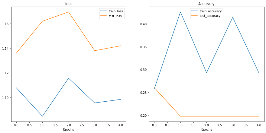
Woah.
Looks like things are all over the place…
But we kind of knew that because our model’s print out results during training didn’t show much promise.
You could try training the model for longer and see what happens when you plot a loss curve over a longer time horizon.
Looking at training and test loss curves is a great way to see if your model is overfitting.
An overfitting model is one that performs better (often by a considerable margin) on the training set than the validation/test set.
If your training loss is far lower than your test loss, your model is overfitting.
As in, it’s learning the patterns in the training too well and those patterns aren’t generalizing to the test data.
The other side is when your training and test loss are not as low as you’d like, this is considered underfitting.
The ideal position for a training and test loss curve is for them to line up closely with each other.
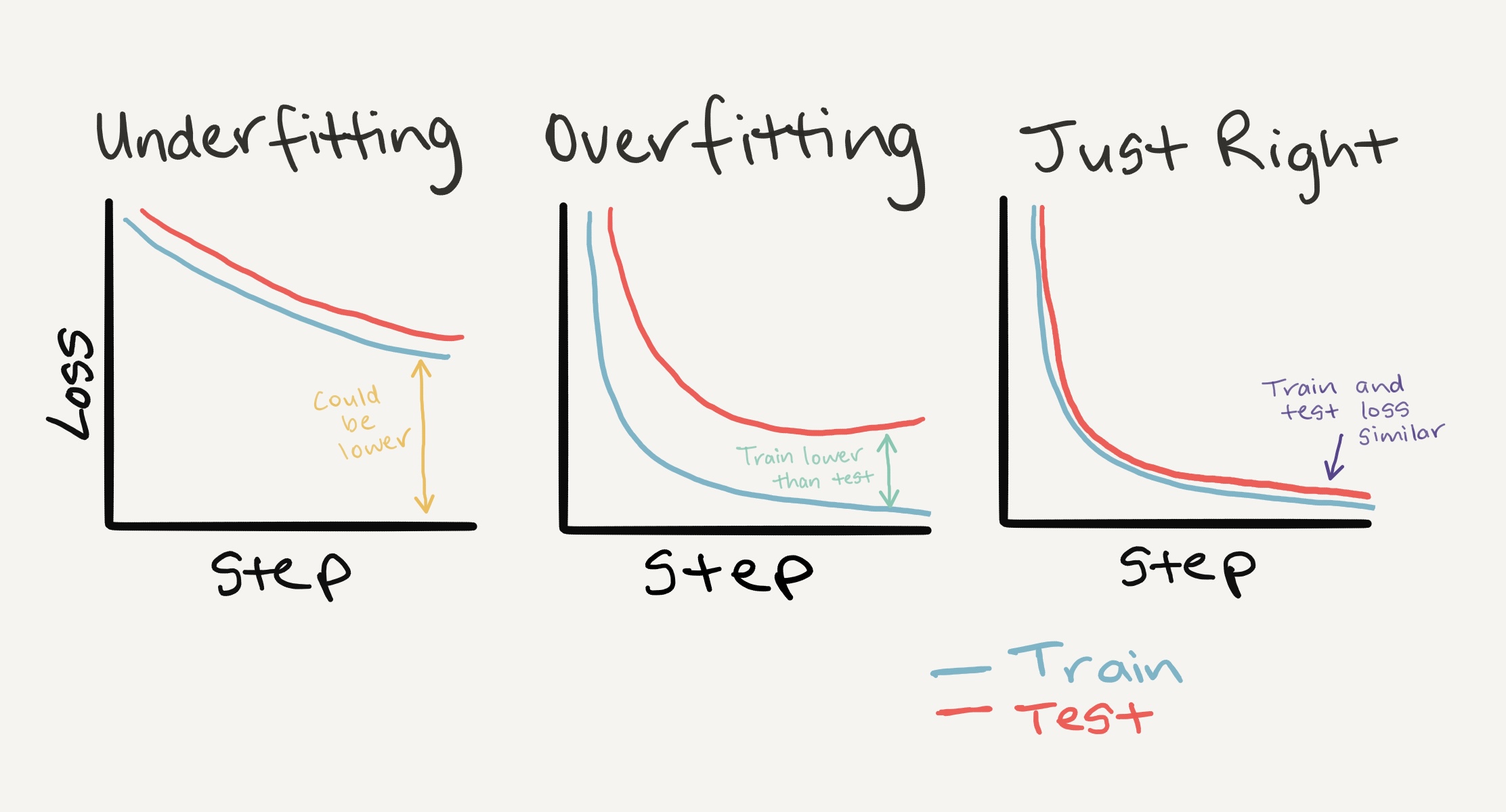
Left: If your training and test loss curves aren’t as low as you’d like, this is considered underfitting. Middle:* When your test/validation loss is higher than your training loss this is considered overfitting. Right: The ideal scenario is when your training and test loss curves line up over time. This means your model is generalizing well. There are more combinations and different things loss curves can do, for more on these, see Google’s Interpreting Loss Curves guide.*
Since the main problem with overfitting is that you’re model is fitting the training data too well, you’ll want to use techniques to “reign it in”.
A common technique of preventing overfitting is known as regularization.
I like to think of this as “making our models more regular”, as in, capable of fitting more kinds of data.
Let’s discuss a few methods to prevent overfitting.
| Method to prevent overfitting | What is it? |
|---|---|
| Get more data | Having more data gives the model more opportunities to learn patterns, patterns which may be more generalizable to new examples. |
| Simplify your model | If the current model is already overfitting the training data, it may be too complicated of a model. This means it’s learning the patterns of the data too well and isn’t able to generalize well to unseen data. One way to simplify a model is to reduce the number of layers it uses or to reduce the number of hidden units in each layer. |
| Use data augmentation | Data augmentation manipulates the training data in a way so that’s harder for the model to learn as it artificially adds more variety to the data. If a model is able to learn patterns in augmented data, the model may be able to generalize better to unseen data. |
| Use transfer learning | Transfer learning involves leveraging the patterns (also called pretrained weights) one model has learned to use as the foundation for your own task. In our case, we could use one computer vision model pretrained on a large variety of images and then tweak it slightly to be more specialized for food images. |
| Use dropout layers | Dropout layers randomly remove connections between hidden layers in neural networks, effectively simplifying a model but also making the remaining connections better. See torch.nn.Dropout() for more. |
| Use learning rate decay | The idea here is to slowly decrease the learning rate as a model trains. This is akin to reaching for a coin at the back of a couch. The closer you get, the smaller your steps. The same with the learning rate, the closer you get to convergence, the smaller you’ll want your weight updates to be. |
| Use early stopping | Early stopping stops model training before it begins to overfit. As in, say the model’s loss has stopped decreasing for the past 10 epochs (this number is arbitrary), you may want to stop the model training here and go with the model weights that had the lowest loss (10 epochs prior). |
There are more methods for dealing with overfitting but these are some of the main ones.
As you start to build more and more deep models, you’ll find because deep learnings are so good at learning patterns in data, dealing with overfitting is one of the primary problems of deep learning.
모델이 과소적합(underfitting) 상태라면 훈련 및 테스트 세트에서 예측 능력이 떨어지는 것으로 간주됩니다.
본질적으로 과소적합 모델은 손실 값을 원하는 수준으로 줄이는 데 실패합니다.
현재 손실 곡선을 보았을 때, 우리의 TinyVGG 모델인 model_0은 데이터에 과소적합된 것으로 보입니다.
과소적합을 처리하는 주요 아이디어는 모델의 예측 능력을 높이는 것입니다.
이를 위한 몇 가지 방법이 있습니다.
| 과소적합 방지 방법 | 설명 |
|---|---|
| 모델에 더 많은 레이어/유닛 추가 | 모델이 과소적합 상태라면, 예측력을 갖추기 위해 필요한 데이터의 패턴/가중치/표현을 학습할 능력이 부족할 수 있습니다. 모델에 더 많은 예측 능력을 추가하는 한 가지 방법은 은닉 레이어의 수나 해당 레이어 내의 유닛 수를 늘리는 것입니다. |
| 학습률 조정 | 아마 모델의 학습률이 처음부터 너무 높을 수 있습니다. 그래서 에포크마다 가중치를 너무 많이 업데이트하려고 시도하여 결국 아무것도 배우지 못하게 됩니다. 이 경우 학습률을 낮추고 어떤 일이 일어나는지 지켜볼 수 있습니다. |
| 전이 학습 사용 | 전이 학습은 과적합과 과소적합 모두를 방지할 수 있습니다. 이미 작동하는 모델의 패턴을 가져와 자신의 문제에 맞게 조정하는 것입니다. |
| 더 오래 훈련 | 때로는 모델이 데이터의 표현을 학습하는 데 더 많은 시간이 필요할 수 있습니다. 소규모 실험에서 모델이 아무것도 학습하지 못한다면, 더 많은 에포크 동안 훈련시키는 것이 더 나은 성능으로 이어질 수 있습니다. |
| 정규화 줄이기 | 과적합을 너무 많이 방지하려고 노력하다 보니 모델이 과소적합되었을 수 있습니다. 정규화 기술을 조금 줄이면 모델이 데이터에 더 잘 맞도록 도울 수 있습니다. |
위에서 논의한 방법 중 어떤 것도 만능 해결책은 아니며, 항상 작동하는 것은 아닙니다.
과적합과 과소적합을 방지하는 것은 머신러닝 연구에서 아마도 가장 활발한 분야일 것입니다.
모든 사람이 자신의 모델이 더 잘 맞기를 원하지만(과소적합 감소), 실세계에서 일반화되지 못할 정도로 잘 맞기를 원하지는 않기 때문입니다(과적합 감소).
과적합과 과소적합 사이에는 미세한 경계가 있습니다.
각각이 너무 지나치면 다른 쪽을 유발할 수 있기 때문입니다.
전이 학습은 자신의 문제에 대한 과적합과 과소적합 문제를 모두 다룰 때 가장 강력한 기술 중 하나일 것입니다.
서로 다른 과적합 및 과소적합 기술을 직접 하나하나 만들 필요 없이, 전이 학습을 사용하면 자신의 문제 공간과 유사한 문제 공간에서 이미 작동하는 모델(예: paperswithcode.com/sota 또는 Hugging Face 모델에서 제공하는 모델)을 가져와 자신의 데이터셋에 적용할 수 있습니다.
나중 노트북에서 전이 학습의 위력을 보게 될 것입니다.
이제 다른 모델을 시도해 볼 시간입니다!
이번에는 데이터를 로드하고 데이터 증강을 사용하여 결과가 개선되는지 확인해 보겠습니다.
먼저 transforms.TrivialAugmentWide() 뿐만 아니라 이미지 크기 조정 및 텐서 변환을 포함하도록 훈련용 변환을 구성하겠습니다.
테스트용 변환도 데이터 증강만 제외하고 동일하게 수행하겠습니다.
# TrivialAugment를 포함한 훈련 변환 생성
train_transform_trivial_augment = transforms.Compose([
    transforms.Resize((64, 64)),
    transforms.TrivialAugmentWide(num_magnitude_bins=31),
    transforms.ToTensor()
])

# 테스트 변환 생성 (데이터 증강 미포함)
test_transform = transforms.Compose([
    transforms.Resize((64, 64)),
    transforms.ToTensor()
])
멋지네요!
이제 torchvision.datasets.ImageFolder()를 사용하여 이미지를 Dataset으로 변환한 다음, torch.utils.data.DataLoader()를 사용하여 DataLoader로 변환하겠습니다.
Dataset 및 DataLoader 생성훈련용 Dataset은 train_transform_trivial_augment를 사용하고 테스트용 Dataset은 test_transform을 사용하도록 하겠습니다.
# Turn image folders into Datasets
train_data_augmented = datasets.ImageFolder(train_dir, transform=train_transform_trivial_augment)
test_data_simple = datasets.ImageFolder(test_dir, transform=test_transform)

train_data_augmented, test_data_simple
(Dataset ImageFolder
Number of datapoints: 225
Root location: data\pizza_steak_sushi\train
StandardTransform
Transform: Compose(
Resize(size=(64, 64), interpolation=bilinear, max_size=None, antialias=None)
TrivialAugmentWide(num_magnitude_bins=31, interpolation=InterpolationMode.NEAREST, fill=None)
ToTensor()
),
Dataset ImageFolder
Number of datapoints: 75
Root location: data\pizza_steak_sushi\test
StandardTransform
Transform: Compose(
Resize(size=(64, 64), interpolation=bilinear, max_size=None, antialias=None)
ToTensor()
))And we’ll make DataLoader’s with a batch_size=32 and with num_workers set to the number of CPUs available on our machine (we can get this using Python’s os.cpu_count()).
# Turn Datasets into DataLoader's
import os
BATCH_SIZE = 32
NUM_WORKERS = os.cpu_count()

torch.manual_seed(42)
train_dataloader_augmented = DataLoader(train_data_augmented,
                                        batch_size=BATCH_SIZE,
                                        shuffle=True,
                                        num_workers=NUM_WORKERS)

test_dataloader_simple = DataLoader(test_data_simple,
                                    batch_size=BATCH_SIZE,
                                    shuffle=False,
                                    num_workers=NUM_WORKERS)

train_dataloader_augmented, test_dataloader
(<torch.utils.data.dataloader.DataLoader at 0x1fd2d0531c0>,
<torch.utils.data.dataloader.DataLoader at 0x1fd2cf94dc0>)Data loaded!
Now to build our next model, model_1, we can reuse our TinyVGG class from before.
We’ll make sure to send it to the target device.
# Create model_1 and send it to the target device
torch.manual_seed(42)
model_1 = TinyVGG(
    input_shape=3,
    hidden_units=10,
    output_shape=len(train_data_augmented.classes)).to(device)
model_1
TinyVGG(
(conv_block_1): Sequential(
(0): Conv2d(3, 10, kernel_size=(3, 3), stride=(1, 1), padding=(1, 1))
(1): ReLU()
(2): Conv2d(10, 10, kernel_size=(3, 3), stride=(1, 1), padding=(1, 1))
(3): ReLU()
(4): MaxPool2d(kernel_size=2, stride=2, padding=0, dilation=1, ceil_mode=False)
)
(conv_block_2): Sequential(
(0): Conv2d(10, 10, kernel_size=(3, 3), stride=(1, 1), padding=(1, 1))
(1): ReLU()
(2): Conv2d(10, 10, kernel_size=(3, 3), stride=(1, 1), padding=(1, 1))
(3): ReLU()
(4): MaxPool2d(kernel_size=2, stride=2, padding=0, dilation=1, ceil_mode=False)
)
(classifier): Sequential(
(0): Flatten(start_dim=1, end_dim=-1)
(1): Linear(in_features=2560, out_features=3, bias=True)
)
)Model ready!
Time to train!
Since we’ve already got functions for the training loop (train_step()) and testing loop (test_step()) and a function to put them together in train(), let’s reuse those.
We’ll use the same setup as model_0 with only the train_dataloader parameter varying: * Train for 5 epochs. * Use train_dataloader=train_dataloader_augmented as the training data in train(). * Use torch.nn.CrossEntropyLoss() as the loss function (since we’re working with multi-class classification). * Use torch.optim.Adam() with lr=0.001 as the learning rate as the optimizer.
# Set random seeds
torch.manual_seed(42)
torch.cuda.manual_seed(42)

# Set number of epochs
NUM_EPOCHS = 5

# Setup loss function and optimizer
loss_fn = nn.CrossEntropyLoss()
optimizer = torch.optim.Adam(params=model_1.parameters(), lr=0.001)

# Start the timer
from timeit import default_timer as timer
start_time = timer()

# Train model_1
model_1_results = train(model=model_1,
                        train_dataloader=train_dataloader_augmented,
                        test_dataloader=test_dataloader_simple,
                        optimizer=optimizer,
                        loss_fn=loss_fn,
                        epochs=NUM_EPOCHS)

# End the timer and print out how long it took
end_time = timer()
print(f"Total training time: {end_time-start_time:.3f} seconds")
Epoch: 1 | train_loss: 1.1074 | train_acc: 0.2461 | test_loss: 1.1058 | test_acc: 0.2604
Epoch: 2 | train_loss: 1.0791 | train_acc: 0.4258 | test_loss: 1.1382 | test_acc: 0.2604
Epoch: 3 | train_loss: 1.0804 | train_acc: 0.4258 | test_loss: 1.1683 | test_acc: 0.2604
Epoch: 4 | train_loss: 1.1287 | train_acc: 0.3047 | test_loss: 1.1626 | test_acc: 0.2604
Epoch: 5 | train_loss: 1.0884 | train_acc: 0.4258 | test_loss: 1.1481 | test_acc: 0.2604
Total training time: 67.543 secondsHmm…
It doesn’t look like our model performed very well again.
Let’s check out its loss curves.
Since we’ve got the results of model_1 saved in a results dictionary, model_1_results, we can plot them using plot_loss_curves().
plot_loss_curves(model_1_results)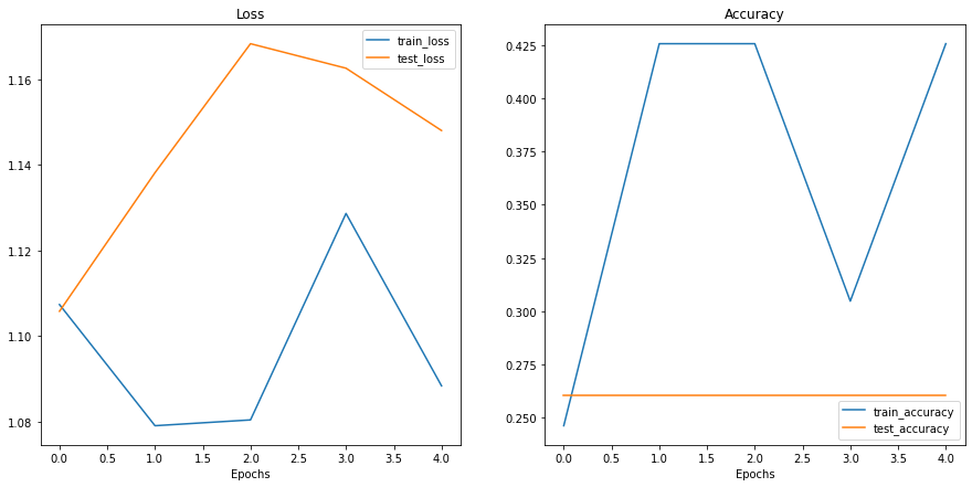
Wow…
These don’t look very good either…
Is our model underfitting or overfitting?
Or both?
Ideally we’d like it have higher accuracy and lower loss right?
What are some methods you could try to use to achieve these?
Even though our models our performing quite poorly, we can still write code to compare them.
Let’s first turn our model results in pandas DataFrames.
import pandas as pd
model_0_df = pd.DataFrame(model_0_results)
model_1_df = pd.DataFrame(model_1_results)
model_0_df| train_loss | train_acc | test_loss | test_acc | |
|---|---|---|---|---|
| 0 | 1.107832 | 0.257812 | 1.136025 | 0.260417 |
| 1 | 1.084726 | 0.425781 | 1.161953 | 0.197917 |
| 2 | 1.115656 | 0.292969 | 1.169479 | 0.197917 |
| 3 | 1.095543 | 0.414062 | 1.137993 | 0.197917 |
| 4 | 1.098464 | 0.292969 | 1.142002 | 0.197917 |
이제 matplotlib을 사용하여 model_0과 model_1의 결과를 함께 시각화하는 플로팅 코드를 작성해 보겠습니다.
# Setup a plot
plt.figure(figsize=(15, 10))

# Get number of epochs
epochs = range(len(model_0_df))

# Plot train loss
plt.subplot(2, 2, 1)
plt.plot(epochs, model_0_df["train_loss"], label="Model 0")
plt.plot(epochs, model_1_df["train_loss"], label="Model 1")
plt.title("Train Loss")
plt.xlabel("Epochs")
plt.legend()

# Plot test loss
plt.subplot(2, 2, 2)
plt.plot(epochs, model_0_df["test_loss"], label="Model 0")
plt.plot(epochs, model_1_df["test_loss"], label="Model 1")
plt.title("Test Loss")
plt.xlabel("Epochs")
plt.legend()

# Plot train accuracy
plt.subplot(2, 2, 3)
plt.plot(epochs, model_0_df["train_acc"], label="Model 0")
plt.plot(epochs, model_1_df["train_acc"], label="Model 1")
plt.title("Train Accuracy")
plt.xlabel("Epochs")
plt.legend()

# Plot test accuracy
plt.subplot(2, 2, 4)
plt.plot(epochs, model_0_df["test_acc"], label="Model 0")
plt.plot(epochs, model_1_df["test_acc"], label="Model 1")
plt.title("Test Accuracy")
plt.xlabel("Epochs")
plt.legend();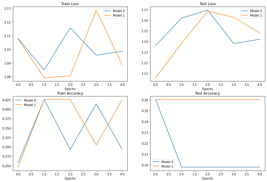
It looks like our models both performed equally poorly and were kind of sporadic (the metrics go up and down sharply).
If you built model_2, what would you do differently to try and improve performance?
If you’ve trained a model on a certain dataset, chances are you’d like to make a prediction on on your own custom data.
In our case, since we’ve trained a model on pizza, steak and sushi images, how could we use our model to make a prediction on one of our own images?
To do so, we can load an image and then preprocess it in a way that matches the type of data our model was trained on.
In other words, we’ll have to convert our own custom image to a tensor and make sure it’s in the right datatype before passing it to our model.
Let’s start by downloading a custom image.
Since our model predicts whether an image contains pizza, steak or sushi, let’s download a photo of my Dad giving two thumbs up to a big pizza from the Learn PyTorch for Deep Learning GitHub.
We download the image using Python’s requests module.
참고: If you’re using Google Colab, you can also upload an image to the current session by going to the left hand side menu -> Files -> Upload to session storage. Beware though, this image will delete when your Google Colab session ends.
# Download custom image
import requests

# Setup custom image path
custom_image_path = data_path / "04-pizza-dad.jpeg"

# Download the image if it doesn't already exist
if not custom_image_path.is_file():
    with open(custom_image_path, "wb") as f:
        # When downloading from GitHub, need to use the "raw" file link
        request = requests.get("https://raw.githubusercontent.com/mrdbourke/pytorch-deep-learning/main/images/04-pizza-dad.jpeg")
        print(f"Downloading {custom_image_path}...")
        f.write(request.content)
else:
    print(f"{custom_image_path} already exists, skipping download.")
data\04-pizza-dad.jpeg already exists, skipping download.Excellent!
Looks like we’ve got a custom image downloaded and ready to go at data/04-pizza-dad.jpeg.
Time to load it in.
PyTorch’s torchvision has several input and output (“IO” or “io” for short) methods for reading and writing images and video in torchvision.io.
Since we want to load in an image, we’ll use torchvision.io.read_image().
This method will read a JPEG or PNG image and turn it into a 3 dimensional RGB or grayscale torch.Tensor with values of datatype uint8 in range [0, 255].
Let’s try it out.
import torchvision

# Read in custom image
custom_image_uint8 = torchvision.io.read_image(str(custom_image_path))

# Print out image data
print(f"Custom image tensor:\n{custom_image_uint8}\n")
print(f"Custom image shape: {custom_image_uint8.shape}\n")
print(f"Custom image dtype: {custom_image_uint8.dtype}")
Custom image tensor:
tensor([[[154, 175, 181, ..., 21, 18, 14],
[146, 167, 180, ..., 21, 18, 15],
[124, 146, 171, ..., 18, 17, 15],
...,
[ 72, 59, 45, ..., 152, 150, 148],
[ 64, 55, 41, ..., 150, 147, 144],
[ 64, 60, 46, ..., 149, 146, 143]],
[[171, 189, 193, ..., 22, 19, 15],
[163, 181, 194, ..., 22, 19, 16],
[141, 163, 185, ..., 19, 18, 16],
...,
[ 55, 42, 28, ..., 106, 104, 102],
[ 47, 38, 24, ..., 108, 105, 102],
[ 47, 43, 29, ..., 107, 104, 101]],
[[117, 138, 145, ..., 17, 14, 10],
[109, 130, 145, ..., 17, 14, 11],
[ 87, 111, 136, ..., 14, 13, 11],
...,
[ 35, 22, 8, ..., 54, 52, 50],
[ 27, 18, 4, ..., 50, 47, 44],
[ 27, 23, 9, ..., 49, 46, 43]]], dtype=torch.uint8)
Custom image shape: torch.Size([3, 4032, 3024])
Custom image dtype: torch.uint8Nice! Looks like our image is in tensor format, however, is this image format compatible with our model?
Our custom_image tensor is of datatype torch.uint8 and its values are between [0, 255].
But our model takes image tensors of datatype torch.float32 and with values between [0, 1].
So before we use our custom image with our model, we’ll need to convert it to the same format as the data our model is trained on.
If we don’t do this, our model will error.
# Try to make a prediction on image in uint8 format (this will error)
model_1.eval()
with torch.inference_mode():
    model_1(custom_image_uint8.to(device))
--------------------------------------------------------------------------- RuntimeError Traceback (most recent call last) Input In [65], in <cell line: 3>() 2 model_1.eval() 3 with torch.inference_mode(): ----> 4 model_1(custom_image_uint8.to(device)) File ~\mambaforge\envs\ds\lib\site-packages\torch\nn\modules\module.py:1110, in Module._call_impl(self, *input, **kwargs) 1106 # If we don't have any hooks, we want to skip the rest of the logic in 1107 # this function, and just call forward. 1108 if not (self._backward_hooks or self._forward_hooks or self._forward_pre_hooks or _global_backward_hooks 1109 or _global_forward_hooks or _global_forward_pre_hooks): -> 1110 return forward_call(*input, **kwargs) 1111 # Do not call functions when jit is used 1112 full_backward_hooks, non_full_backward_hooks = [], [] Input In [45], in TinyVGG.forward(self, x) 39 def forward(self, x: torch.Tensor): ---> 40 x = self.conv_block_1(x) 41 # print(x.shape) 42 x = self.conv_block_2(x) File ~\mambaforge\envs\ds\lib\site-packages\torch\nn\modules\module.py:1110, in Module._call_impl(self, *input, **kwargs) 1106 # If we don't have any hooks, we want to skip the rest of the logic in 1107 # this function, and just call forward. 1108 if not (self._backward_hooks or self._forward_hooks or self._forward_pre_hooks or _global_backward_hooks 1109 or _global_forward_hooks or _global_forward_pre_hooks): -> 1110 return forward_call(*input, **kwargs) 1111 # Do not call functions when jit is used 1112 full_backward_hooks, non_full_backward_hooks = [], [] File ~\mambaforge\envs\ds\lib\site-packages\torch\nn\modules\container.py:141, in Sequential.forward(self, input) 139 def forward(self, input): 140 for module in self: --> 141 input = module(input) 142 return input File ~\mambaforge\envs\ds\lib\site-packages\torch\nn\modules\module.py:1110, in Module._call_impl(self, *input, **kwargs) 1106 # If we don't have any hooks, we want to skip the rest of the logic in 1107 # this function, and just call forward. 1108 if not (self._backward_hooks or self._forward_hooks or self._forward_pre_hooks or _global_backward_hooks 1109 or _global_forward_hooks or _global_forward_pre_hooks): -> 1110 return forward_call(*input, **kwargs) 1111 # Do not call functions when jit is used 1112 full_backward_hooks, non_full_backward_hooks = [], [] File ~\mambaforge\envs\ds\lib\site-packages\torch\nn\modules\conv.py:447, in Conv2d.forward(self, input) 446 def forward(self, input: Tensor) -> Tensor: --> 447 return self._conv_forward(input, self.weight, self.bias) File ~\mambaforge\envs\ds\lib\site-packages\torch\nn\modules\conv.py:443, in Conv2d._conv_forward(self, input, weight, bias) 439 if self.padding_mode != 'zeros': 440 return F.conv2d(F.pad(input, self._reversed_padding_repeated_twice, mode=self.padding_mode), 441 weight, bias, self.stride, 442 _pair(0), self.dilation, self.groups) --> 443 return F.conv2d(input, weight, bias, self.stride, 444 self.padding, self.dilation, self.groups) RuntimeError: Input type (torch.cuda.ByteTensor) and weight type (torch.cuda.FloatTensor) should be the same
If we try to make a prediction on an image in a different datatype to what our model was trained on, we get an error like the following:
RuntimeError: Input type (torch.cuda.ByteTensor) and weight type (torch.cuda.FloatTensor) should be the same
Let’s fix this by converting our custom image to the same datatype as what our model was trained on (torch.float32).
# Load in custom image and convert the tensor values to float32
custom_image = torchvision.io.read_image(str(custom_image_path)).type(torch.float32)

# Divide the image pixel values by 255 to get them between [0, 1]
custom_image = custom_image / 255.

# Print out image data
print(f"Custom image tensor:\n{custom_image}\n")
print(f"Custom image shape: {custom_image.shape}\n")
print(f"Custom image dtype: {custom_image.dtype}")
Custom image tensor:
tensor([[[0.6039, 0.6863, 0.7098, ..., 0.0824, 0.0706, 0.0549],
[0.5725, 0.6549, 0.7059, ..., 0.0824, 0.0706, 0.0588],
[0.4863, 0.5725, 0.6706, ..., 0.0706, 0.0667, 0.0588],
...,
[0.2824, 0.2314, 0.1765, ..., 0.5961, 0.5882, 0.5804],
[0.2510, 0.2157, 0.1608, ..., 0.5882, 0.5765, 0.5647],
[0.2510, 0.2353, 0.1804, ..., 0.5843, 0.5725, 0.5608]],
[[0.6706, 0.7412, 0.7569, ..., 0.0863, 0.0745, 0.0588],
[0.6392, 0.7098, 0.7608, ..., 0.0863, 0.0745, 0.0627],
[0.5529, 0.6392, 0.7255, ..., 0.0745, 0.0706, 0.0627],
...,
[0.2157, 0.1647, 0.1098, ..., 0.4157, 0.4078, 0.4000],
[0.1843, 0.1490, 0.0941, ..., 0.4235, 0.4118, 0.4000],
[0.1843, 0.1686, 0.1137, ..., 0.4196, 0.4078, 0.3961]],
[[0.4588, 0.5412, 0.5686, ..., 0.0667, 0.0549, 0.0392],
[0.4275, 0.5098, 0.5686, ..., 0.0667, 0.0549, 0.0431],
[0.3412, 0.4353, 0.5333, ..., 0.0549, 0.0510, 0.0431],
...,
[0.1373, 0.0863, 0.0314, ..., 0.2118, 0.2039, 0.1961],
[0.1059, 0.0706, 0.0157, ..., 0.1961, 0.1843, 0.1725],
[0.1059, 0.0902, 0.0353, ..., 0.1922, 0.1804, 0.1686]]])
Custom image shape: torch.Size([3, 4032, 3024])
Custom image dtype: torch.float32Beautiful, it looks like our image data is now in the same format our model was trained on.
Except for one thing…
It’s shape.
Our model was trained on images with shape [3, 64, 64], whereas our custom image is currently [3, 4032, 3024].
How could we make sure our custom image is the same shape as the images our model was trained on?
Are there any torchvision.transforms that could help?
Before we answer that question, let’s plot the image with matplotlib to make sure it looks okay, remember we’ll have to permute the dimensions from CHW to HWC to suit matplotlib’s requirements.
# Plot custom image
plt.imshow(custom_image.permute(1, 2, 0)) # need to permute image dimensions from CHW -> HWC otherwise matplotlib will error
plt.title(f"Image shape: {custom_image.shape}")
plt.axis(False);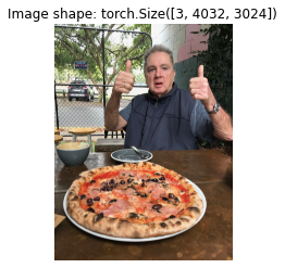
Two thumbs up!
Now how could we get our image to be the same size as the images our model was trained on?
One way to do so is with torchvision.transforms.Resize().
Let’s compose a transform pipeline to do so.
# Create transform pipleine to resize image
custom_image_transform = transforms.Compose([
    transforms.Resize((64, 64)),
])

# Transform target image
custom_image_transformed = custom_image_transform(custom_image)

# Print out original shape and new shape
print(f"Original shape: {custom_image.shape}")
print(f"New shape: {custom_image_transformed.shape}")
Original shape: torch.Size([3, 4032, 3024])
New shape: torch.Size([3, 64, 64])Woohoo!
Let’s finally make a prediction on our own custom image.
model_1.eval()
with torch.inference_mode():
    custom_image_pred = model_1(custom_image_transformed)
--------------------------------------------------------------------------- RuntimeError Traceback (most recent call last) Input In [69], in <cell line: 2>() 1 model_1.eval() 2 with torch.inference_mode(): ----> 3 custom_image_pred = model_1(custom_image_transformed) File ~\mambaforge\envs\ds\lib\site-packages\torch\nn\modules\module.py:1110, in Module._call_impl(self, *input, **kwargs) 1106 # If we don't have any hooks, we want to skip the rest of the logic in 1107 # this function, and just call forward. 1108 if not (self._backward_hooks or self._forward_hooks or self._forward_pre_hooks or _global_backward_hooks 1109 or _global_forward_hooks or _global_forward_pre_hooks): -> 1110 return forward_call(*input, **kwargs) 1111 # Do not call functions when jit is used 1112 full_backward_hooks, non_full_backward_hooks = [], [] Input In [45], in TinyVGG.forward(self, x) 39 def forward(self, x: torch.Tensor): ---> 40 x = self.conv_block_1(x) 41 # print(x.shape) 42 x = self.conv_block_2(x) File ~\mambaforge\envs\ds\lib\site-packages\torch\nn\modules\module.py:1110, in Module._call_impl(self, *input, **kwargs) 1106 # If we don't have any hooks, we want to skip the rest of the logic in 1107 # this function, and just call forward. 1108 if not (self._backward_hooks or self._forward_hooks or self._forward_pre_hooks or _global_backward_hooks 1109 or _global_forward_hooks or _global_forward_pre_hooks): -> 1110 return forward_call(*input, **kwargs) 1111 # Do not call functions when jit is used 1112 full_backward_hooks, non_full_backward_hooks = [], [] File ~\mambaforge\envs\ds\lib\site-packages\torch\nn\modules\container.py:141, in Sequential.forward(self, input) 139 def forward(self, input): 140 for module in self: --> 141 input = module(input) 142 return input File ~\mambaforge\envs\ds\lib\site-packages\torch\nn\modules\module.py:1110, in Module._call_impl(self, *input, **kwargs) 1106 # If we don't have any hooks, we want to skip the rest of the logic in 1107 # this function, and just call forward. 1108 if not (self._backward_hooks or self._forward_hooks or self._forward_pre_hooks or _global_backward_hooks 1109 or _global_forward_hooks or _global_forward_pre_hooks): -> 1110 return forward_call(*input, **kwargs) 1111 # Do not call functions when jit is used 1112 full_backward_hooks, non_full_backward_hooks = [], [] File ~\mambaforge\envs\ds\lib\site-packages\torch\nn\modules\conv.py:447, in Conv2d.forward(self, input) 446 def forward(self, input: Tensor) -> Tensor: --> 447 return self._conv_forward(input, self.weight, self.bias) File ~\mambaforge\envs\ds\lib\site-packages\torch\nn\modules\conv.py:443, in Conv2d._conv_forward(self, input, weight, bias) 439 if self.padding_mode != 'zeros': 440 return F.conv2d(F.pad(input, self._reversed_padding_repeated_twice, mode=self.padding_mode), 441 weight, bias, self.stride, 442 _pair(0), self.dilation, self.groups) --> 443 return F.conv2d(input, weight, bias, self.stride, 444 self.padding, self.dilation, self.groups) RuntimeError: Expected all tensors to be on the same device, but found at least two devices, cpu and cuda:0! (when checking argument for argument weight in method wrapper___slow_conv2d_forward)
Oh my goodness…
Despite our preparations our custom image and model are on different devices.
And we get the error:
RuntimeError: Expected all tensors to be on the same device, but found at least two devices, cpu and cuda:0! (when checking argument for argument weight in method wrapper___slow_conv2d_forward)
Let’s fix that by putting our custom_image_transformed on the target device.
model_1.eval()
with torch.inference_mode():
    custom_image_pred = model_1(custom_image_transformed.to(device))
--------------------------------------------------------------------------- RuntimeError Traceback (most recent call last) Input In [70], in <cell line: 2>() 1 model_1.eval() 2 with torch.inference_mode(): ----> 3 custom_image_pred = model_1(custom_image_transformed.to(device)) File ~\mambaforge\envs\ds\lib\site-packages\torch\nn\modules\module.py:1110, in Module._call_impl(self, *input, **kwargs) 1106 # If we don't have any hooks, we want to skip the rest of the logic in 1107 # this function, and just call forward. 1108 if not (self._backward_hooks or self._forward_hooks or self._forward_pre_hooks or _global_backward_hooks 1109 or _global_forward_hooks or _global_forward_pre_hooks): -> 1110 return forward_call(*input, **kwargs) 1111 # Do not call functions when jit is used 1112 full_backward_hooks, non_full_backward_hooks = [], [] Input In [45], in TinyVGG.forward(self, x) 42 x = self.conv_block_2(x) 43 # print(x.shape) ---> 44 x = self.classifier(x) 45 # print(x.shape) 46 return x File ~\mambaforge\envs\ds\lib\site-packages\torch\nn\modules\module.py:1110, in Module._call_impl(self, *input, **kwargs) 1106 # If we don't have any hooks, we want to skip the rest of the logic in 1107 # this function, and just call forward. 1108 if not (self._backward_hooks or self._forward_hooks or self._forward_pre_hooks or _global_backward_hooks 1109 or _global_forward_hooks or _global_forward_pre_hooks): -> 1110 return forward_call(*input, **kwargs) 1111 # Do not call functions when jit is used 1112 full_backward_hooks, non_full_backward_hooks = [], [] File ~\mambaforge\envs\ds\lib\site-packages\torch\nn\modules\container.py:141, in Sequential.forward(self, input) 139 def forward(self, input): 140 for module in self: --> 141 input = module(input) 142 return input File ~\mambaforge\envs\ds\lib\site-packages\torch\nn\modules\module.py:1110, in Module._call_impl(self, *input, **kwargs) 1106 # If we don't have any hooks, we want to skip the rest of the logic in 1107 # this function, and just call forward. 1108 if not (self._backward_hooks or self._forward_hooks or self._forward_pre_hooks or _global_backward_hooks 1109 or _global_forward_hooks or _global_forward_pre_hooks): -> 1110 return forward_call(*input, **kwargs) 1111 # Do not call functions when jit is used 1112 full_backward_hooks, non_full_backward_hooks = [], [] File ~\mambaforge\envs\ds\lib\site-packages\torch\nn\modules\linear.py:103, in Linear.forward(self, input) 102 def forward(self, input: Tensor) -> Tensor: --> 103 return F.linear(input, self.weight, self.bias) RuntimeError: mat1 and mat2 shapes cannot be multiplied (10x256 and 2560x3)
What now?
It looks like we’re getting a shape error.
Why might this be?
We converted our custom image to be the same size as the images our model was trained on…
Oh wait…
There’s one dimension we forgot about.
The batch size.
Our model expects image tensors with a batch size dimension at the start (NCHW where N is the batch size).
Except our custom image is currently only CHW.
We can add a batch size dimension using torch.unsqueeze(dim=0) to add an extra dimension our image and finally make a prediction.
Essentially we’ll be telling our model to predict on a single image (an image with a batch_size of 1).
model_1.eval()
with torch.inference_mode():
    # Add an extra dimension to image
    custom_image_transformed_with_batch_size = custom_image_transformed.unsqueeze(dim=0)

    # Print out different shapes
    print(f"Custom image transformed shape: {custom_image_transformed.shape}")
    print(f"Unsqueezed custom image shape: {custom_image_transformed_with_batch_size.shape}")

    # Make a prediction on image with an extra dimension
    custom_image_pred = model_1(custom_image_transformed.unsqueeze(dim=0).to(device))
Custom image transformed shape: torch.Size([3, 64, 64])
Unsqueezed custom image shape: torch.Size([1, 3, 64, 64])Yes!!!
It looks like it worked!
참고: What we’ve just gone through are three of the classical and most common deep learning and PyTorch issues: 1. Wrong datatypes - our model expects
torch.float32where our original custom image wasuint8. 2. Wrong device - our model was on the targetdevice(in our case, the GPU) whereas our target data hadn’t been moved to the targetdeviceyet. 3. Wrong shapes - our model expected an input image of shape[N, C, H, W]or[batch_size, color_channels, height, width]whereas our custom image tensor was of shape[color_channels, height, width].Keep in mind, these errors aren’t just for predicting on custom images.
They will be present with almost every kind of data type (text, audio, structured data) and problem you work with.
Now let’s take a look at our model’s predictions.
custom_image_predtensor([[ 0.1161, 0.0213, -0.1422]], device='cuda:0')Alright, these are still in logit form (the raw outputs of a model are called logits).
Let’s convert them from logits -> prediction probabilities -> prediction labels.
# Print out prediction logits
print(f"Prediction logits: {custom_image_pred}")

# Convert logits -> prediction probabilities (using torch.softmax() for multi-class classification)
custom_image_pred_probs = torch.softmax(custom_image_pred, dim=1)
print(f"Prediction probabilities: {custom_image_pred_probs}")

# Convert prediction probabilities -> prediction labels
custom_image_pred_label = torch.argmax(custom_image_pred_probs, dim=1)
print(f"Prediction label: {custom_image_pred_label}")
Prediction logits: tensor([[ 0.1161, 0.0213, -0.1422]], device='cuda:0')
Prediction probabilities: tensor([[0.3729, 0.3392, 0.2880]], device='cuda:0')
Prediction label: tensor([0], device='cuda:0')Alright!
Looking good.
But of course our prediction label is still in index/tensor form.
We can convert it to a string class name prediction by indexing on the class_names list.
# Find the predicted label
custom_image_pred_class = class_names[custom_image_pred_label.cpu()] # put pred label to CPU, otherwise will error
custom_image_pred_class'pizza'Wow.
It looks like the model gets the prediction right, even though it was performing poorly based on our evaluation metrics.
참고: The model in its current form will predict “pizza”, “steak” or “sushi” no matter what image it’s given. If you wanted your model to predict on a different class, you’d have to train it to do so.
But if we check the custom_image_pred_probs, we’ll notice that the model gives almost equal weight (the values are similar) to every class.
# The values of the prediction probabilities are quite similar
custom_image_pred_probs
tensor([[0.3729, 0.3392, 0.2880]], device='cuda:0')Having prediction probabilities this similar could mean a couple of things: 1. The model is trying to predict all three classes at the same time (there may be an image containing pizza, steak and sushi). 2. The model doesn’t really know what it wants to predict and is in turn just assigning similar values to each of the classes.
Our case is number 2, since our model is poorly trained, it is basically guessing the prediction.
Doing all of the above steps every time you’d like to make a prediction on a custom image would quickly become tedious.
So let’s put them all together in a function we can easily use over and over again.
Specifically, let’s make a function that: 1. Takes in a target image path and converts to the right datatype for our model (torch.float32). 2. Makes sure the target image pixel values are in the range [0, 1]. 3. Transforms the target image if necessary. 4. Makes sure the model is on the target device. 5. Makes a prediction on the target image with a trained model (ensuring the image is the right size and on the same device as the model). 6. Converts the model’s output logits to prediction probabilities. 7. Converts the prediction probabilities to prediction labels. 8. Plots the target image alongside the model prediction and prediction probability.
A fair few steps but we’ve got this!
def pred_and_plot_image(model: torch.nn.Module,
                        image_path: str,
                        class_names: List[str] = None,
                        transform=None,
                        device: torch.device = device):
    """Makes a prediction on a target image and plots the image with its prediction."""

    # 1. Load in image and convert the tensor values to float32
    target_image = torchvision.io.read_image(str(image_path)).type(torch.float32)

    # 2. Divide the image pixel values by 255 to get them between [0, 1]
    target_image = target_image / 255.

    # 3. Transform if necessary
    if transform:
        target_image = transform(target_image)

    # 4. Make sure the model is on the target device
    model.to(device)

    # 5. Turn on model evaluation mode and inference mode
    model.eval()
    with torch.inference_mode():
        # Add an extra dimension to the image
        target_image = target_image.unsqueeze(dim=0)

        # Make a prediction on image with an extra dimension and send it to the target device
        target_image_pred = model(target_image.to(device))

    # 6. Convert logits -> prediction probabilities (using torch.softmax() for multi-class classification)
    target_image_pred_probs = torch.softmax(target_image_pred, dim=1)

    # 7. Convert prediction probabilities -> prediction labels
    target_image_pred_label = torch.argmax(target_image_pred_probs, dim=1)

    # 8. Plot the image alongside the prediction and prediction probability
    plt.imshow(target_image.squeeze().permute(1, 2, 0)) # make sure it's the right size for matplotlib
    if class_names:
        title = f"Pred: {class_names[target_image_pred_label.cpu()]} | Prob: {target_image_pred_probs.max().cpu():.3f}"
    else:
        title = f"Pred: {target_image_pred_label} | Prob: {target_image_pred_probs.max().cpu():.3f}"
    plt.title(title)
    plt.axis(False);
What a nice looking function, let’s test it out.
# Pred on our custom image
pred_and_plot_image(model=model_1,
                    image_path=custom_image_path,
                    class_names=class_names,
                    transform=custom_image_transform,
                    device=device)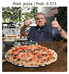
Two thumbs up again!
Looks like our model got the prediction right just by guessing.
This won’t always be the case with other images though…
The image is pixelated too because we resized it to [64, 64] using custom_image_transform.
Exercise: Try making a prediction with one of your own images of pizza, steak or sushi and see what happens.
We’ve covered a fair bit in this module.
Let’s summarise it with a few dot points.
torch.utils.data.Dataset.torch.utils.data.DataLoader’s in PyTorch help turn your Dataset’s into iterables that can be used when training and testing a model.torch.float32 when your data is torch.uint8.[batch_size, color_channels, height, width] when your data is [color_channels, height, width].All of the exercises are focused on practicing the code in the sections above.
You should be able to complete them by referencing each section or by following the resource(s) linked.
All exercises should be completed using device-agnostic code.
Resources: * Exercise template notebook for 04 * Example solutions notebook for 04 (try the exercises before looking at this)
DataLoader’s ready to use.model_0 we built in section 7.model_0.torch.optim.Adam() with a learning rate of 0.001 as the optimizer.Dataset’s and DataLoader’s through PyTorch datasets and dataloaders tutorial notebook.torchvision.transforms documentation.
torchvision.datasets documentation.