(tensor([[[0.0000, 0.0000, 0.0000, 0.0000, 0.0000, 0.0000, 0.0000, 0.0000,
0.0000, 0.0000, 0.0000, 0.0000, 0.0000, 0.0000, 0.0000, 0.0000,
0.0000, 0.0000, 0.0000, 0.0000, 0.0000, 0.0000, 0.0000, 0.0000,
0.0000, 0.0000, 0.0000, 0.0000],
[0.0000, 0.0000, 0.0000, 0.0000, 0.0000, 0.0000, 0.0000, 0.0000,
0.0000, 0.0000, 0.0000, 0.0000, 0.0000, 0.0000, 0.0000, 0.0000,
0.0000, 0.0000, 0.0000, 0.0000, 0.0000, 0.0000, 0.0000, 0.0000,
0.0000, 0.0000, 0.0000, 0.0000],
[0.0000, 0.0000, 0.0000, 0.0000, 0.0000, 0.0000, 0.0000, 0.0000,
0.0000, 0.0000, 0.0000, 0.0000, 0.0000, 0.0000, 0.0000, 0.0000,
0.0000, 0.0000, 0.0000, 0.0000, 0.0000, 0.0000, 0.0000, 0.0000,
0.0000, 0.0000, 0.0000, 0.0000],
[0.0000, 0.0000, 0.0000, 0.0000, 0.0000, 0.0000, 0.0000, 0.0000,
0.0000, 0.0000, 0.0000, 0.0000, 0.0039, 0.0000, 0.0000, 0.0510,
0.2863, 0.0000, 0.0000, 0.0039, 0.0157, 0.0000, 0.0000, 0.0000,
0.0000, 0.0039, 0.0039, 0.0000],
[0.0000, 0.0000, 0.0000, 0.0000, 0.0000, 0.0000, 0.0000, 0.0000,
0.0000, 0.0000, 0.0000, 0.0000, 0.0118, 0.0000, 0.1412, 0.5333,
0.4980, 0.2431, 0.2118, 0.0000, 0.0000, 0.0000, 0.0039, 0.0118,
0.0157, 0.0000, 0.0000, 0.0118],
[0.0000, 0.0000, 0.0000, 0.0000, 0.0000, 0.0000, 0.0000, 0.0000,
0.0000, 0.0000, 0.0000, 0.0000, 0.0235, 0.0000, 0.4000, 0.8000,
0.6902, 0.5255, 0.5647, 0.4824, 0.0902, 0.0000, 0.0000, 0.0000,
0.0000, 0.0471, 0.0392, 0.0000],
[0.0000, 0.0000, 0.0000, 0.0000, 0.0000, 0.0000, 0.0000, 0.0000,
0.0000, 0.0000, 0.0000, 0.0000, 0.0000, 0.0000, 0.6078, 0.9255,
0.8118, 0.6980, 0.4196, 0.6118, 0.6314, 0.4275, 0.2510, 0.0902,
0.3020, 0.5098, 0.2824, 0.0588],
[0.0000, 0.0000, 0.0000, 0.0000, 0.0000, 0.0000, 0.0000, 0.0000,
0.0000, 0.0000, 0.0000, 0.0039, 0.0000, 0.2706, 0.8118, 0.8745,
0.8549, 0.8471, 0.8471, 0.6392, 0.4980, 0.4745, 0.4784, 0.5725,
0.5529, 0.3451, 0.6745, 0.2588],
[0.0000, 0.0000, 0.0000, 0.0000, 0.0000, 0.0000, 0.0000, 0.0000,
0.0000, 0.0039, 0.0039, 0.0039, 0.0000, 0.7843, 0.9098, 0.9098,
0.9137, 0.8980, 0.8745, 0.8745, 0.8431, 0.8353, 0.6431, 0.4980,
0.4824, 0.7686, 0.8980, 0.0000],
[0.0000, 0.0000, 0.0000, 0.0000, 0.0000, 0.0000, 0.0000, 0.0000,
0.0000, 0.0000, 0.0000, 0.0000, 0.0000, 0.7176, 0.8824, 0.8471,
0.8745, 0.8941, 0.9216, 0.8902, 0.8784, 0.8706, 0.8784, 0.8667,
0.8745, 0.9608, 0.6784, 0.0000],
[0.0000, 0.0000, 0.0000, 0.0000, 0.0000, 0.0000, 0.0000, 0.0000,
0.0000, 0.0000, 0.0000, 0.0000, 0.0000, 0.7569, 0.8941, 0.8549,
0.8353, 0.7765, 0.7059, 0.8314, 0.8235, 0.8275, 0.8353, 0.8745,
0.8627, 0.9529, 0.7922, 0.0000],
[0.0000, 0.0000, 0.0000, 0.0000, 0.0000, 0.0000, 0.0000, 0.0000,
0.0000, 0.0039, 0.0118, 0.0000, 0.0471, 0.8588, 0.8627, 0.8314,
0.8549, 0.7529, 0.6627, 0.8902, 0.8157, 0.8549, 0.8784, 0.8314,
0.8863, 0.7725, 0.8196, 0.2039],
[0.0000, 0.0000, 0.0000, 0.0000, 0.0000, 0.0000, 0.0000, 0.0000,
0.0000, 0.0000, 0.0235, 0.0000, 0.3882, 0.9569, 0.8706, 0.8627,
0.8549, 0.7961, 0.7765, 0.8667, 0.8431, 0.8353, 0.8706, 0.8627,
0.9608, 0.4667, 0.6549, 0.2196],
[0.0000, 0.0000, 0.0000, 0.0000, 0.0000, 0.0000, 0.0000, 0.0000,
0.0000, 0.0157, 0.0000, 0.0000, 0.2157, 0.9255, 0.8941, 0.9020,
0.8941, 0.9412, 0.9098, 0.8353, 0.8549, 0.8745, 0.9176, 0.8510,
0.8510, 0.8196, 0.3608, 0.0000],
[0.0000, 0.0000, 0.0039, 0.0157, 0.0235, 0.0275, 0.0078, 0.0000,
0.0000, 0.0000, 0.0000, 0.0000, 0.9294, 0.8863, 0.8510, 0.8745,
0.8706, 0.8588, 0.8706, 0.8667, 0.8471, 0.8745, 0.8980, 0.8431,
0.8549, 1.0000, 0.3020, 0.0000],
[0.0000, 0.0118, 0.0000, 0.0000, 0.0000, 0.0000, 0.0000, 0.0000,
0.0000, 0.2431, 0.5686, 0.8000, 0.8941, 0.8118, 0.8353, 0.8667,
0.8549, 0.8157, 0.8275, 0.8549, 0.8784, 0.8745, 0.8588, 0.8431,
0.8784, 0.9569, 0.6235, 0.0000],
[0.0000, 0.0000, 0.0000, 0.0000, 0.0706, 0.1725, 0.3216, 0.4196,
0.7412, 0.8941, 0.8627, 0.8706, 0.8510, 0.8863, 0.7843, 0.8039,
0.8275, 0.9020, 0.8784, 0.9176, 0.6902, 0.7373, 0.9804, 0.9725,
0.9137, 0.9333, 0.8431, 0.0000],
[0.0000, 0.2235, 0.7333, 0.8157, 0.8784, 0.8667, 0.8784, 0.8157,
0.8000, 0.8392, 0.8157, 0.8196, 0.7843, 0.6235, 0.9608, 0.7569,
0.8078, 0.8745, 1.0000, 1.0000, 0.8667, 0.9176, 0.8667, 0.8275,
0.8627, 0.9098, 0.9647, 0.0000],
[0.0118, 0.7922, 0.8941, 0.8784, 0.8667, 0.8275, 0.8275, 0.8392,
0.8039, 0.8039, 0.8039, 0.8627, 0.9412, 0.3137, 0.5882, 1.0000,
0.8980, 0.8667, 0.7373, 0.6039, 0.7490, 0.8235, 0.8000, 0.8196,
0.8706, 0.8941, 0.8824, 0.0000],
[0.3843, 0.9137, 0.7765, 0.8235, 0.8706, 0.8980, 0.8980, 0.9176,
0.9765, 0.8627, 0.7608, 0.8431, 0.8510, 0.9451, 0.2549, 0.2863,
0.4157, 0.4588, 0.6588, 0.8588, 0.8667, 0.8431, 0.8510, 0.8745,
0.8745, 0.8784, 0.8980, 0.1137],
[0.2941, 0.8000, 0.8314, 0.8000, 0.7569, 0.8039, 0.8275, 0.8824,
0.8471, 0.7255, 0.7725, 0.8078, 0.7765, 0.8353, 0.9412, 0.7647,
0.8902, 0.9608, 0.9373, 0.8745, 0.8549, 0.8314, 0.8196, 0.8706,
0.8627, 0.8667, 0.9020, 0.2627],
[0.1882, 0.7961, 0.7176, 0.7608, 0.8353, 0.7725, 0.7255, 0.7451,
0.7608, 0.7529, 0.7922, 0.8392, 0.8588, 0.8667, 0.8627, 0.9255,
0.8824, 0.8471, 0.7804, 0.8078, 0.7294, 0.7098, 0.6941, 0.6745,
0.7098, 0.8039, 0.8078, 0.4510],
[0.0000, 0.4784, 0.8588, 0.7569, 0.7020, 0.6706, 0.7176, 0.7686,
0.8000, 0.8235, 0.8353, 0.8118, 0.8275, 0.8235, 0.7843, 0.7686,
0.7608, 0.7490, 0.7647, 0.7490, 0.7765, 0.7529, 0.6902, 0.6118,
0.6549, 0.6941, 0.8235, 0.3608],
[0.0000, 0.0000, 0.2902, 0.7412, 0.8314, 0.7490, 0.6863, 0.6745,
0.6863, 0.7098, 0.7255, 0.7373, 0.7412, 0.7373, 0.7569, 0.7765,
0.8000, 0.8196, 0.8235, 0.8235, 0.8275, 0.7373, 0.7373, 0.7608,
0.7529, 0.8471, 0.6667, 0.0000],
[0.0078, 0.0000, 0.0000, 0.0000, 0.2588, 0.7843, 0.8706, 0.9294,
0.9373, 0.9490, 0.9647, 0.9529, 0.9569, 0.8667, 0.8627, 0.7569,
0.7490, 0.7020, 0.7137, 0.7137, 0.7098, 0.6902, 0.6510, 0.6588,
0.3882, 0.2275, 0.0000, 0.0000],
[0.0000, 0.0000, 0.0000, 0.0000, 0.0000, 0.0000, 0.0000, 0.1569,
0.2392, 0.1725, 0.2824, 0.1608, 0.1373, 0.0000, 0.0000, 0.0000,
0.0000, 0.0000, 0.0000, 0.0000, 0.0000, 0.0000, 0.0000, 0.0000,
0.0000, 0.0000, 0.0000, 0.0000],
[0.0000, 0.0000, 0.0000, 0.0000, 0.0000, 0.0000, 0.0000, 0.0000,
0.0000, 0.0000, 0.0000, 0.0000, 0.0000, 0.0000, 0.0000, 0.0000,
0.0000, 0.0000, 0.0000, 0.0000, 0.0000, 0.0000, 0.0000, 0.0000,
0.0000, 0.0000, 0.0000, 0.0000],
[0.0000, 0.0000, 0.0000, 0.0000, 0.0000, 0.0000, 0.0000, 0.0000,
0.0000, 0.0000, 0.0000, 0.0000, 0.0000, 0.0000, 0.0000, 0.0000,
0.0000, 0.0000, 0.0000, 0.0000, 0.0000, 0.0000, 0.0000, 0.0000,
0.0000, 0.0000, 0.0000, 0.0000]]]),
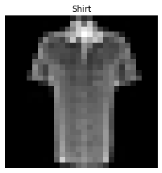
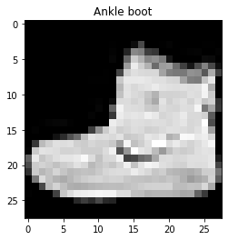
9)
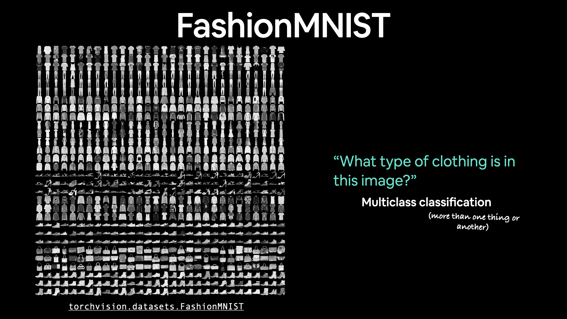
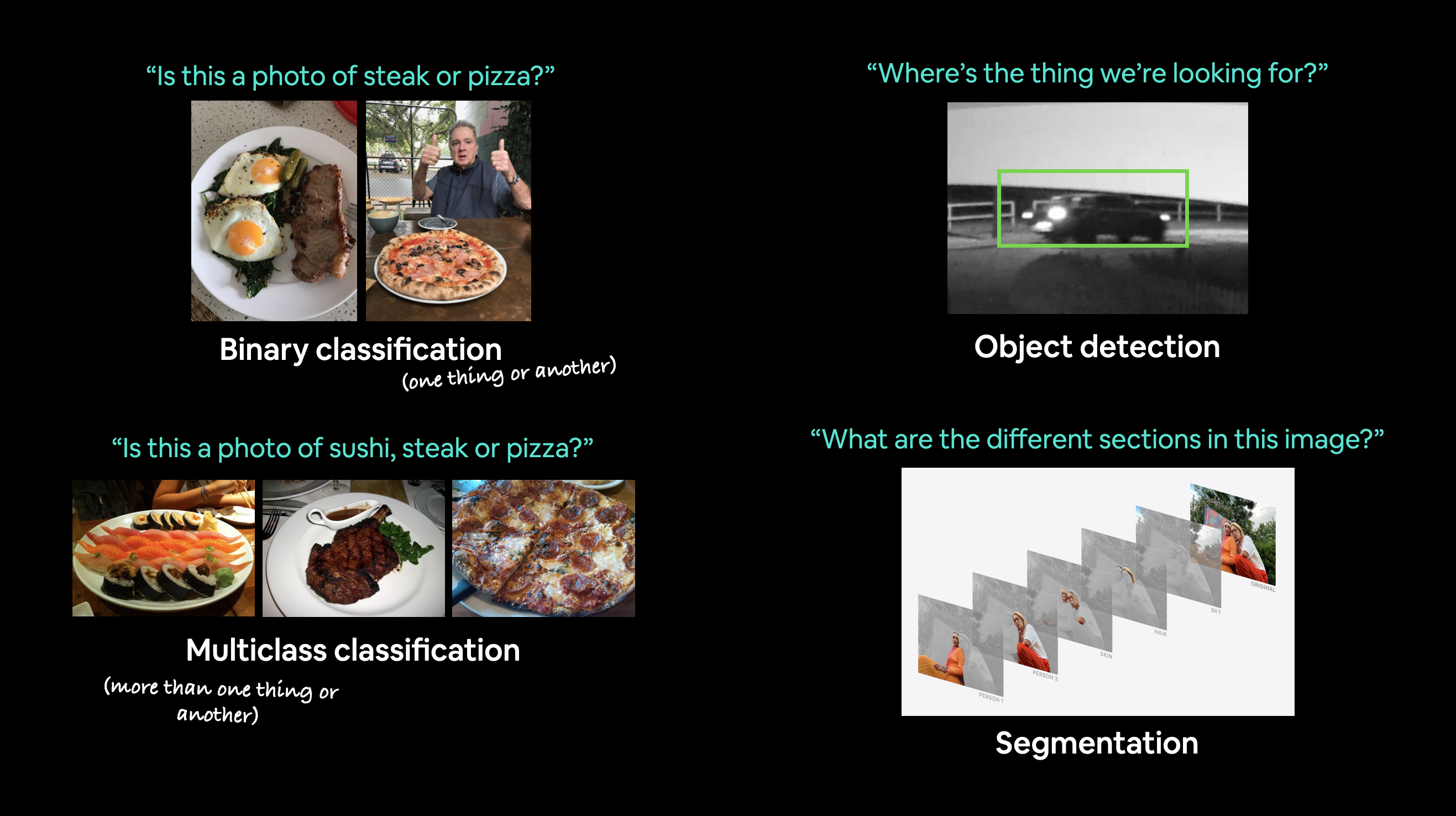 이진 분류, 다중 클래스 분류, 객체 탐지 및 분할에 대한 컴퓨터 비전 문제 예시입니다.
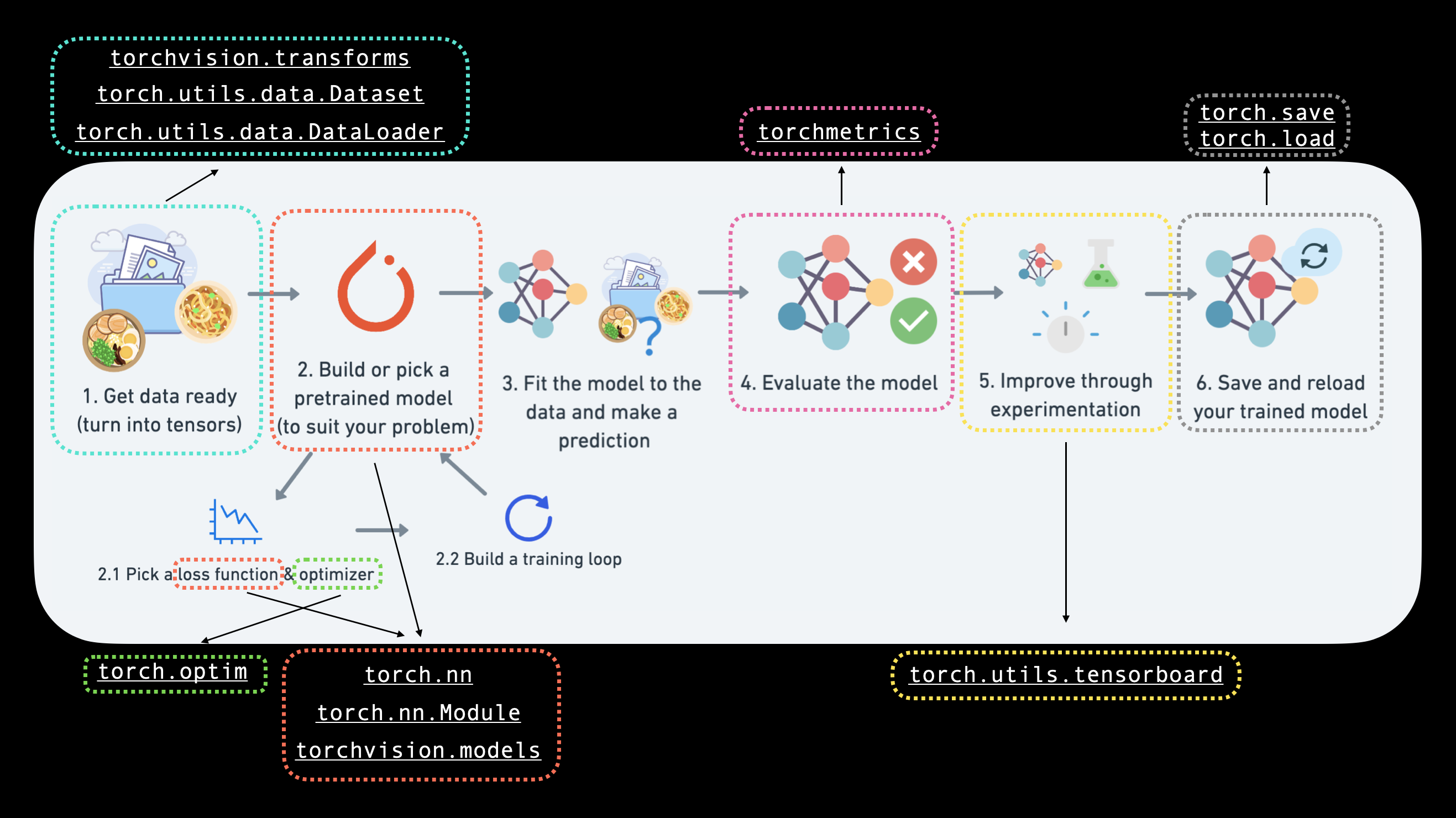
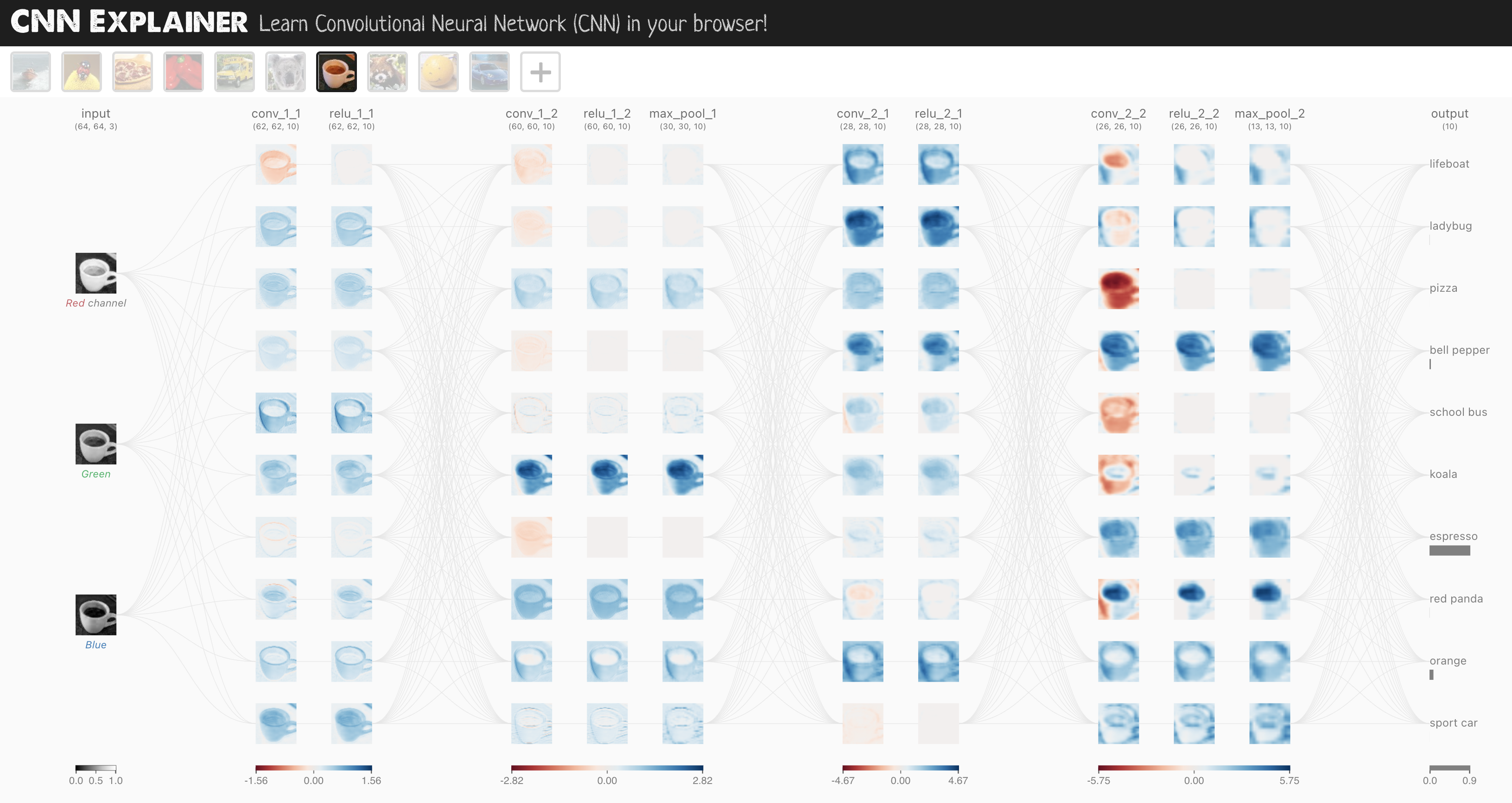
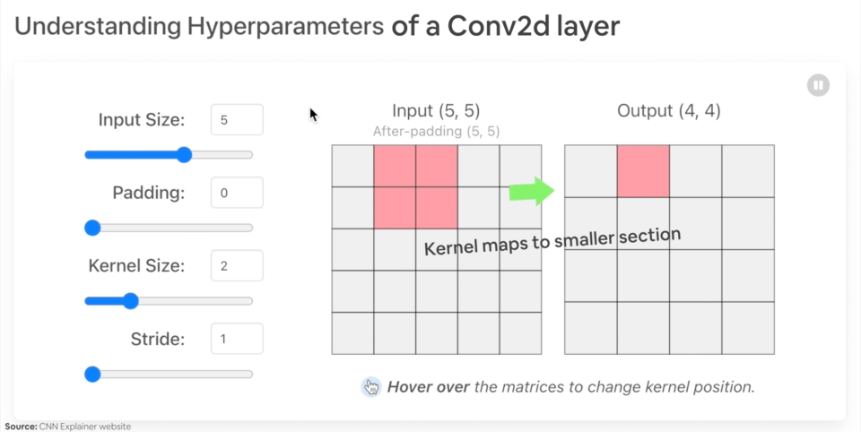
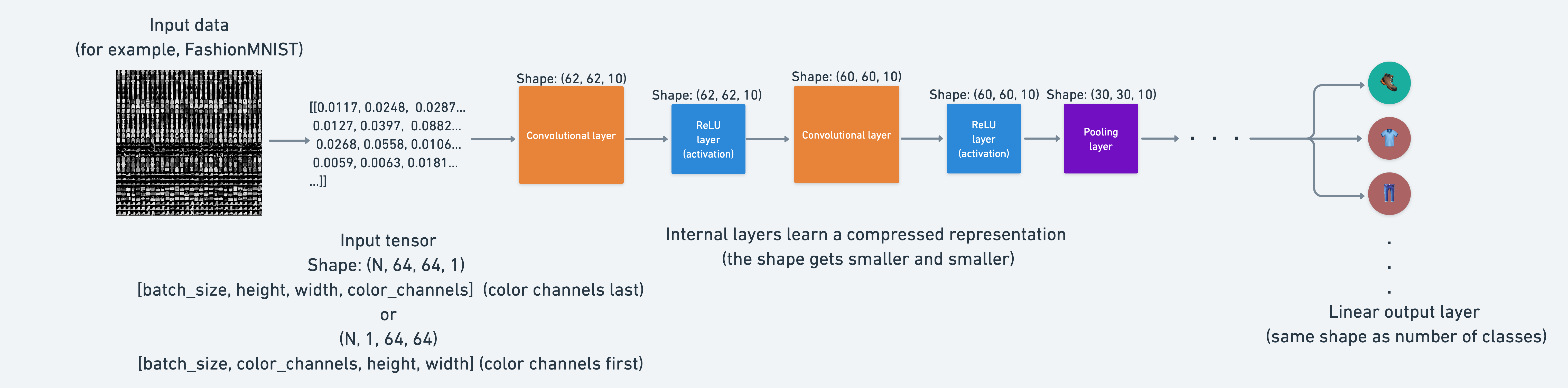
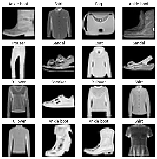
 다양한 문제에는 다양한 입력 및 출력 모양이 있습니다. 하지만 전제는 동일합니다. 데이터를 숫자로 인코딩하고, 해당 숫자에서 패턴을 찾기 위한 모델을 구축하고, 그 패턴을 의미 있는 것으로 변환하는 것입니다.
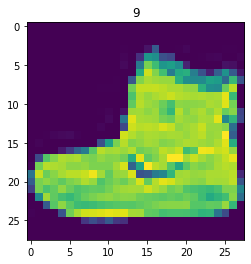
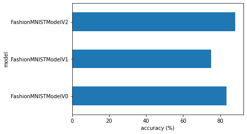
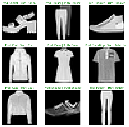
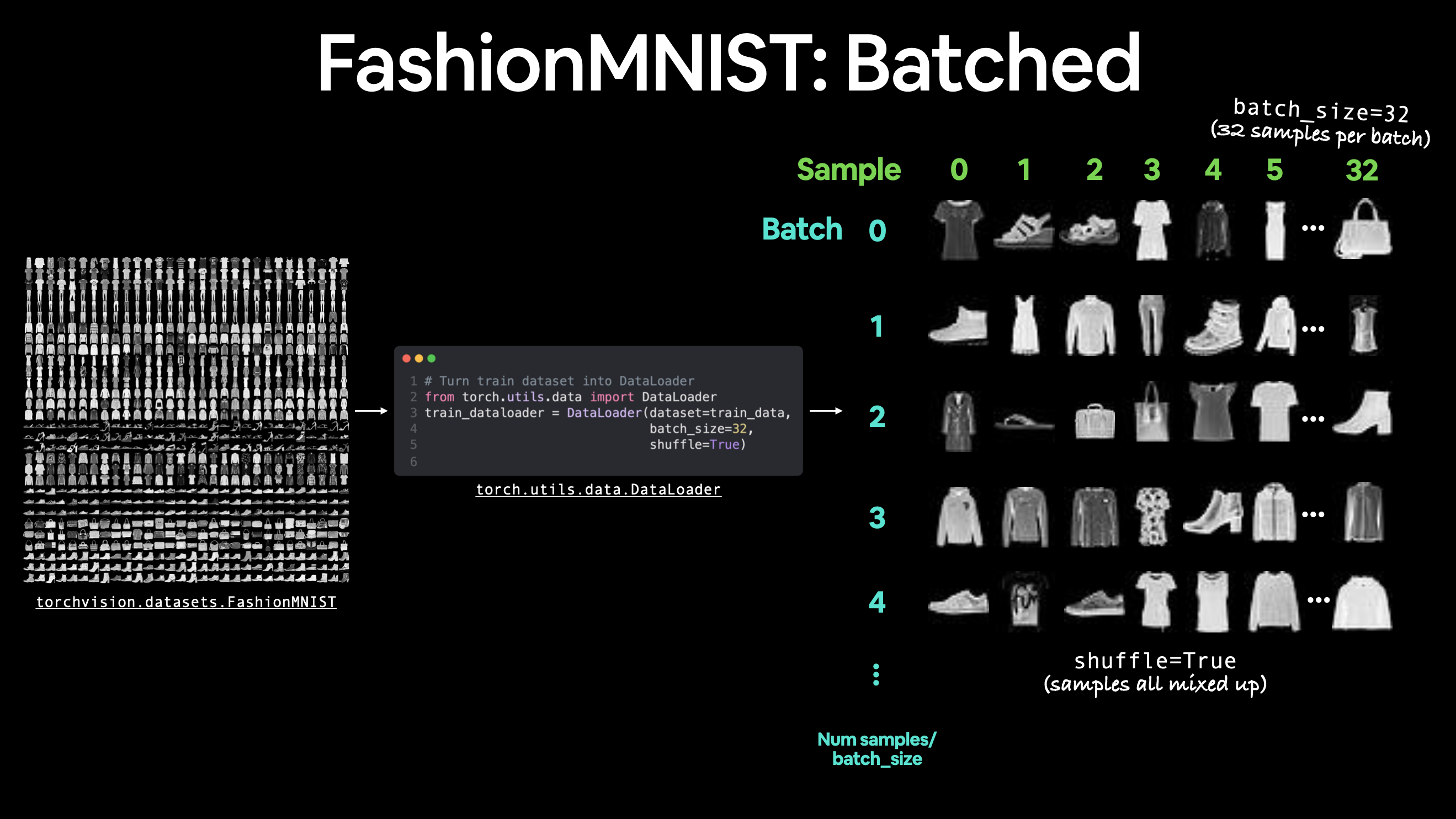 FashionMNIST를 배치 크기 32로 배치하고 셔플을 켠 모습입니다. 다른 데이터셋에 대해서도 유사한 배치 프로세스가 발생하지만 배치 크기에 따라 달라집니다.