실제 뉴스, 웹 로그, 영화 평점 데이터를 활용하여 배운 기술들을 통합 적용합니다.
import warnings'ignore' )from numpy.random import randnimport numpy as np123 )import osimport matplotlib.pyplot as pltimport pandas as pd# Matplotlib 한글 폰트 설정 (macOS용) 'font' , family= 'AppleGothic' )'axes' , unicode_minus= False )"figure" , figsize= (10 , 6 ))= 4 )= 20 = 20 = 80
= "datasets/bitly_usagov/example.txt"
Bitly 데이터셋
URL 단축 서비스 로그 데이터를 분석해 봅니다.
import jsonwith open (path) as f:= [json.loads(line) for line in f]
Bitly 데이터 분석
대규모 로그 데이터에서 의미 있는 통계를 추출하는 과정을 실습합니다.
= [rec["tz" ] for rec in records]
---------------------------------------------------------------------------
KeyError Traceback (most recent call last)
Cell In[4] , line 1
----> 1 time_zones = [ rec [ " tz " ] for rec in records ]
Cell In[4] , line 1 , in <listcomp> (.0)
----> 1 time_zones = [rec [ " tz " ] for rec in records]
KeyError : 'tz'
= [rec["tz" ] for rec in records if "tz" in rec]10 ]
['America/New_York',
 'America/Denver',
 'America/New_York',
 'America/Sao_Paulo',
 'America/New_York',
 'America/New_York',
 'Europe/Warsaw',
 '',
 '',
 '']
def get_counts(sequence):= {}for x in sequence:if x in counts:+= 1 else := 1 return counts
from collections import defaultdictdef get_counts2(sequence):= defaultdict(int ) # values will initialize to 0 for x in sequence:+= 1 return counts
= get_counts(time_zones)"America/New_York" ]len (time_zones)
def top_counts(count_dict, n= 10 ):= [(count, tz) for tz, count in count_dict.items()]return value_key_pairs[- n:]
[(33, 'America/Sao_Paulo'),
 (35, 'Europe/Madrid'),
 (36, 'Pacific/Honolulu'),
 (37, 'Asia/Tokyo'),
 (74, 'Europe/London'),
 (191, 'America/Denver'),
 (382, 'America/Los_Angeles'),
 (400, 'America/Chicago'),
 (521, ''),
 (1251, 'America/New_York')]
from collections import Counter= Counter(time_zones)10 )
[('America/New_York', 1251),
 ('', 521),
 ('America/Chicago', 400),
 ('America/Los_Angeles', 382),
 ('America/Denver', 191),
 ('Europe/London', 74),
 ('Asia/Tokyo', 37),
 ('Pacific/Honolulu', 36),
 ('Europe/Madrid', 35),
 ('America/Sao_Paulo', 33)]
= pd.DataFrame(records)
"tz" ].head()
<class 'pandas.core.frame.DataFrame'>
RangeIndex: 3560 entries, 0 to 3559
Data columns (total 18 columns):
 #   Column       Non-Null Count  Dtype
---  ------       --------------  -----
 0   a            3440 non-null   object
 1   c            2919 non-null   object
 2   nk           3440 non-null   float64
 3   tz           3440 non-null   object
 4   gr           2919 non-null   object
 5   g            3440 non-null   object
 6   h            3440 non-null   object
 7   l            3440 non-null   object
 8   al           3094 non-null   object
 9   hh           3440 non-null   object
 10  r            3440 non-null   object
 11  u            3440 non-null   object
 12  t            3440 non-null   float64
 13  hc           3440 non-null   float64
 14  cy           2919 non-null   object
 15  ll           2919 non-null   object
 16  _heartbeat_  120 non-null    float64
 17  kw           93 non-null     object
dtypes: float64(4), object(14)
memory usage: 500.8+ KB
0     America/New_York
1       America/Denver
2     America/New_York
3    America/Sao_Paulo
4     America/New_York
Name: tz, dtype: object
= frame["tz" ].value_counts()
tz
America/New_York       1251
                        521
America/Chicago         400
America/Los_Angeles     382
America/Denver          191
Name: count, dtype: int64
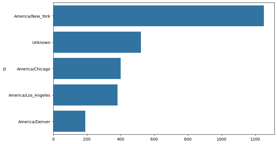
= frame["tz" ].fillna("Missing" )== "" ] = "Unknown" = clean_tz.value_counts()
tz
America/New_York       1251
Unknown                 521
America/Chicago         400
America/Los_Angeles     382
America/Denver          191
Name: count, dtype: int64
= (10 , 4 ))
<Figure size 1000x400 with 0 Axes>
<Figure size 1000x400 with 0 Axes>
import seaborn as sns= tz_counts.head()= subset.index, x= subset.to_numpy())
"a" ][1 ]"a" ][50 ]"a" ][51 ][:50 ] # 긴 줄
'Mozilla/5.0 (Linux; U; Android 2.2.2; en-us; LG-P9'
= pd.Series([x.split()[0 ] for x in frame["a" ].dropna()])5 )8 )
Mozilla/5.0                 2594
Mozilla/4.0                  601
GoogleMaps/RochesterNY       121
Opera/9.80                    34
TEST_INTERNET_AGENT           24
GoogleProducer                21
Mozilla/6.0                    5
BlackBerry8520/5.0.0.681       4
Name: count, dtype: int64
= frame[frame["a" ].notna()].copy()
"os" ] = np.where(cframe["a" ].str .contains("Windows" ),"Windows" , "Not Windows" )"os" ].head(5 )
0        Windows
1    Not Windows
2        Windows
3    Not Windows
4        Windows
Name: os, dtype: object
= cframe.groupby(["tz" , "os" ])
= by_tz_os.size().unstack().fillna(0 )
tz
245.0
276.0
Africa/Cairo
0.0
3.0
Africa/Casablanca
0.0
1.0
Africa/Ceuta
0.0
2.0
Africa/Johannesburg
0.0
1.0
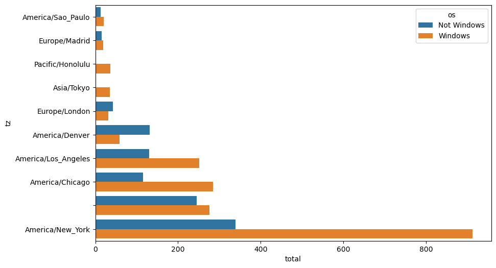
= agg_counts.sum ("columns" ).argsort()10 ]
array([24, 20, 21, 92, 87, 53, 54, 57, 26, 55])
= agg_counts.take(indexer[- 10 :])
tz
America/Sao_Paulo
13.0
20.0
Europe/Madrid
16.0
19.0
Pacific/Honolulu
0.0
36.0
Asia/Tokyo
2.0
35.0
Europe/London
43.0
31.0
America/Denver
132.0
59.0
America/Los_Angeles
130.0
252.0
America/Chicago
115.0
285.0
245.0
276.0
America/New_York
339.0
912.0
sum (axis= "columns" ).nlargest(10 )
tz
America/New_York       1251.0
                        521.0
America/Chicago         400.0
America/Los_Angeles     382.0
America/Denver          191.0
Europe/London            74.0
Asia/Tokyo               37.0
Pacific/Honolulu         36.0
Europe/Madrid            35.0
America/Sao_Paulo        33.0
dtype: float64
<Figure size 1000x600 with 0 Axes>
<Figure size 1000x600 with 0 Axes>
= count_subset.stack()= "total" = count_subset.reset_index()10 )= "total" , y= "tz" , hue= "os" , data= count_subset)
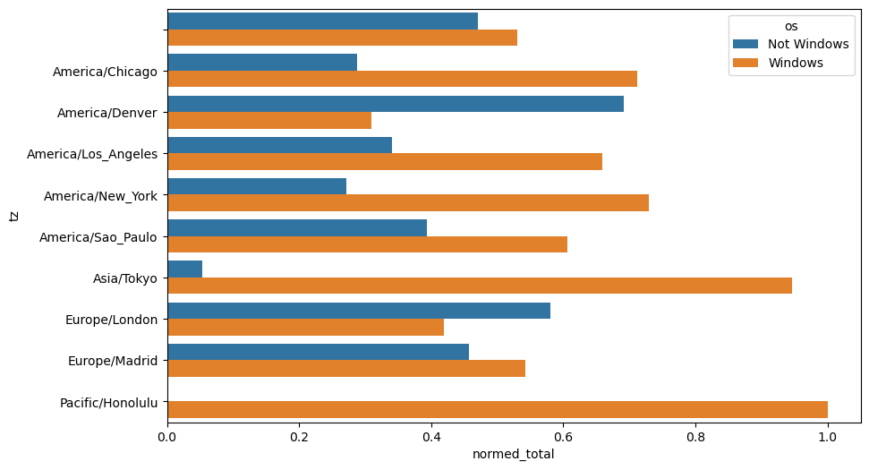
def norm_total(group):"normed_total" ] = group["total" ] / group["total" ].sum ()return group= count_subset.groupby("tz" ).apply (norm_total)
<Figure size 1000x600 with 0 Axes>
<Figure size 1000x600 with 0 Axes>
= "normed_total" , y= "tz" , hue= "os" , data= results)
= count_subset.groupby("tz" )= count_subset["total" ] / g["total" ].transform("sum" )
MovieLens 데이터 분석
사용자 맞춤형 분석을 위한 다중 테이블 결합과 집계 과정을 수행합니다.
= ["user_id" , "gender" , "age" , "occupation" , "zip" ]= pd.read_table("datasets/movielens/users.dat" , sep= "::" ,= None , names= unames, engine= "python" )= ["user_id" , "movie_id" , "rating" , "timestamp" ]= pd.read_table("datasets/movielens/ratings.dat" , sep= "::" ,= None , names= rnames, engine= "python" )= ["movie_id" , "title" , "genres" ]= pd.read_table("datasets/movielens/movies.dat" , sep= "::" ,= None , names= mnames, engine= "python" )
5 )5 )5 )
0
1
1193
5
978300760
1
1
661
3
978302109
2
1
914
3
978301968
3
1
3408
4
978300275
4
1
2355
5
978824291
...
...
...
...
...
1000204
6040
1091
1
956716541
1000205
6040
1094
5
956704887
1000206
6040
562
5
956704746
1000207
6040
1096
4
956715648
1000208
6040
1097
4
956715569
1000209 rows × 4 columns
= pd.merge(pd.merge(ratings, users), movies)0 ]
user_id                                            1
movie_id                                        1193
rating                                             5
timestamp                                  978300760
gender                                             F
age                                                1
occupation                                        10
zip                                            48067
title         One Flew Over the Cuckoo's Nest (1975)
genres                                         Drama
Name: 0, dtype: object
= data.pivot_table("rating" , index= "title" ,= "gender" , aggfunc= "mean" )5 )
title
$1,000,000 Duck (1971)
3.375000
2.761905
'Night Mother (1986)
3.388889
3.352941
'Til There Was You (1997)
2.675676
2.733333
'burbs, The (1989)
2.793478
2.962085
...And Justice for All (1979)
3.828571
3.689024
= data.groupby("title" ).size()= ratings_by_title.index[ratings_by_title >= 250 ]
Index([''burbs, The (1989)', '10 Things I Hate About You (1999)',
       '101 Dalmatians (1961)', '101 Dalmatians (1996)', '12 Angry Men (1957)',
       '13th Warrior, The (1999)', '2 Days in the Valley (1996)',
       '20,000 Leagues Under the Sea (1954)', '2001: A Space Odyssey (1968)',
       '2010 (1984)',
       ...
       'X-Men (2000)', 'Year of Living Dangerously (1982)',
       'Yellow Submarine (1968)', 'You've Got Mail (1998)',
       'Young Frankenstein (1974)', 'Young Guns (1988)',
       'Young Guns II (1990)', 'Young Sherlock Holmes (1985)',
       'Zero Effect (1998)', 'eXistenZ (1999)'],
      dtype='object', name='title', length=1216)
= mean_ratings.loc[active_titles]
title
'burbs, The (1989)
2.793478
2.962085
10 Things I Hate About You (1999)
3.646552
3.311966
101 Dalmatians (1961)
3.791444
3.500000
101 Dalmatians (1996)
3.240000
2.911215
12 Angry Men (1957)
4.184397
4.328421
...
...
...
Young Guns (1988)
3.371795
3.425620
Young Guns II (1990)
2.934783
2.904025
Young Sherlock Holmes (1985)
3.514706
3.363344
Zero Effect (1998)
3.864407
3.723140
eXistenZ (1999)
3.098592
3.289086
1216 rows × 2 columns
= mean_ratings.rename(index= {"Seven Samurai (The Magnificent Seven) (Shichinin no samurai) (1954)" :"Seven Samurai (Shichinin no samurai) (1954)" })
= mean_ratings.sort_values("F" , ascending= False )
title
Close Shave, A (1995)
4.644444
4.473795
Wrong Trousers, The (1993)
4.588235
4.478261
Sunset Blvd. (a.k.a. Sunset Boulevard) (1950)
4.572650
4.464589
Wallace & Gromit: The Best of Aardman Animation (1996)
4.563107
4.385075
Schindler's List (1993)
4.562602
4.491415
"diff" ] = mean_ratings["M" ] - mean_ratings["F" ]
= mean_ratings.sort_values("diff" )
title
Dirty Dancing (1987)
3.790378
2.959596
-0.830782
Jumpin' Jack Flash (1986)
3.254717
2.578358
-0.676359
Grease (1978)
3.975265
3.367041
-0.608224
Little Women (1994)
3.870588
3.321739
-0.548849
Steel Magnolias (1989)
3.901734
3.365957
-0.535777
- 1 ].head()
title
Good, The Bad and The Ugly, The (1966)
3.494949
4.221300
0.726351
Kentucky Fried Movie, The (1977)
2.878788
3.555147
0.676359
Dumb & Dumber (1994)
2.697987
3.336595
0.638608
Longest Day, The (1962)
3.411765
4.031447
0.619682
Cable Guy, The (1996)
2.250000
2.863787
0.613787
= data.groupby("title" )["rating" ].std()= rating_std_by_title.loc[active_titles]
title
'burbs, The (1989)                   1.107760
10 Things I Hate About You (1999)    0.989815
101 Dalmatians (1961)                0.982103
101 Dalmatians (1996)                1.098717
12 Angry Men (1957)                  0.812731
Name: rating, dtype: float64
= False )[:10 ]
title
Dumb & Dumber (1994)                     1.321333
Blair Witch Project, The (1999)          1.316368
Natural Born Killers (1994)              1.307198
Tank Girl (1995)                         1.277695
Rocky Horror Picture Show, The (1975)    1.260177
Eyes Wide Shut (1999)                    1.259624
Evita (1996)                             1.253631
Billy Madison (1995)                     1.249970
Fear and Loathing in Las Vegas (1998)    1.246408
Bicentennial Man (1999)                  1.245533
Name: rating, dtype: float64
"genres" ].head()"genres" ].head().str .split("|" )"genre" ] = movies.pop("genres" ).str .split("|" )
0
1
Toy Story (1995)
[Animation, Children's, Comedy]
1
2
Jumanji (1995)
[Adventure, Children's, Fantasy]
2
3
Grumpier Old Men (1995)
[Comedy, Romance]
3
4
Waiting to Exhale (1995)
[Comedy, Drama]
4
5
Father of the Bride Part II (1995)
[Comedy]
= movies.explode("genre" )10 ]
0
1
Toy Story (1995)
Animation
0
1
Toy Story (1995)
Children's
0
1
Toy Story (1995)
Comedy
1
2
Jumanji (1995)
Adventure
1
2
Jumanji (1995)
Children's
1
2
Jumanji (1995)
Fantasy
2
3
Grumpier Old Men (1995)
Comedy
2
3
Grumpier Old Men (1995)
Romance
3
4
Waiting to Exhale (1995)
Comedy
3
4
Waiting to Exhale (1995)
Drama
= pd.merge(pd.merge(movies_exploded, ratings), users)0 ]= (ratings_with_genre.groupby(["genre" , "age" ])"rating" ].mean()"age" ))10 ]
genre
Action
3.506385
3.447097
3.453358
3.538107
3.528543
3.611333
3.610709
Adventure
3.449975
3.408525
3.443163
3.515291
3.528963
3.628163
3.649064
Animation
3.476113
3.624014
3.701228
3.740545
3.734856
3.780020
3.756233
Children's
3.241642
3.294257
3.426873
3.518423
3.527593
3.556555
3.621822
Comedy
3.497491
3.460417
3.490385
3.561984
3.591789
3.646868
3.650949
Crime
3.710170
3.668054
3.680321
3.733736
3.750661
3.810688
3.832549
Documentary
3.730769
3.865865
3.946690
3.953747
3.966521
3.908108
3.961538
Drama
3.794735
3.721930
3.726428
3.782512
3.784356
3.878415
3.933465
Fantasy
3.317647
3.353778
3.452484
3.482301
3.532468
3.581570
3.532700
Film-Noir
4.145455
3.997368
4.058725
4.064910
4.105376
4.175401
4.125932
! head - n 10 datasets/ babynames/ yob1880.txt
Mary,F,7065
Anna,F,2604
Emma,F,2003
Elizabeth,F,1939
Minnie,F,1746
Margaret,F,1578
Ida,F,1472
Alice,F,1414
Bertha,F,1320
Sarah,F,1288
= pd.read_csv("datasets/babynames/yob1880.txt" ,= ["name" , "sex" , "births" ])
0
Mary
F
7065
1
Anna
F
2604
2
Emma
F
2003
3
Elizabeth
F
1939
4
Minnie
F
1746
...
...
...
...
1995
Woodie
M
5
1996
Worthy
M
5
1997
Wright
M
5
1998
York
M
5
1999
Zachariah
M
5
2000 rows × 3 columns
"sex" )["births" ].sum ()
sex
F     90993
M    110493
Name: births, dtype: int64
= []for year in range (1880 , 2011 ):= f"datasets/babynames/yob { year} .txt" = pd.read_csv(path, names= ["name" , "sex" , "births" ])# Add a column for the year "year" ] = year# Concatenate everything into a single DataFrame = pd.concat(pieces, ignore_index= True )
0
Mary
F
7065
1880
1
Anna
F
2604
1880
2
Emma
F
2003
1880
3
Elizabeth
F
1939
1880
4
Minnie
F
1746
1880
...
...
...
...
...
1690779
Zymaire
M
5
2010
1690780
Zyonne
M
5
2010
1690781
Zyquarius
M
5
2010
1690782
Zyran
M
5
2010
1690783
Zzyzx
M
5
2010
1690784 rows × 4 columns
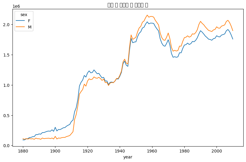
= names.pivot_table("births" , index= "year" ,= "sex" , aggfunc= sum )= "성별 및 연도별 총 출생아 수" )
def add_prop(group):"prop" ] = group["births" ] / group["births" ].sum ()return group= names.groupby(["year" , "sex" ], group_keys= False ).apply (add_prop)
0
Mary
F
7065
1880
0.077643
1
Anna
F
2604
1880
0.028618
2
Emma
F
2003
1880
0.022013
3
Elizabeth
F
1939
1880
0.021309
4
Minnie
F
1746
1880
0.019188
...
...
...
...
...
...
1690779
Zymaire
M
5
2010
0.000003
1690780
Zyonne
M
5
2010
0.000003
1690781
Zyquarius
M
5
2010
0.000003
1690782
Zyran
M
5
2010
0.000003
1690783
Zzyzx
M
5
2010
0.000003
1690784 rows × 5 columns
"year" , "sex" ])["prop" ].sum ()
year  sex
1880  F      1.0
      M      1.0
1881  F      1.0
      M      1.0
1882  F      1.0
            ...
2008  M      1.0
2009  F      1.0
      M      1.0
2010  F      1.0
      M      1.0
Name: prop, Length: 262, dtype: float64
def get_top1000(group):return group.sort_values("births" , ascending= False )[:1000 ]= names.groupby(["year" , "sex" ])= grouped.apply (get_top1000)
year
sex
1880
F
0
Mary
F
7065
1880
0.077643
1
Anna
F
2604
1880
0.028618
2
Emma
F
2003
1880
0.022013
3
Elizabeth
F
1939
1880
0.021309
4
Minnie
F
1746
1880
0.019188
= top1000.reset_index(drop= True )
0
Mary
F
7065
1880
0.077643
1
Anna
F
2604
1880
0.028618
2
Emma
F
2003
1880
0.022013
3
Elizabeth
F
1939
1880
0.021309
4
Minnie
F
1746
1880
0.019188
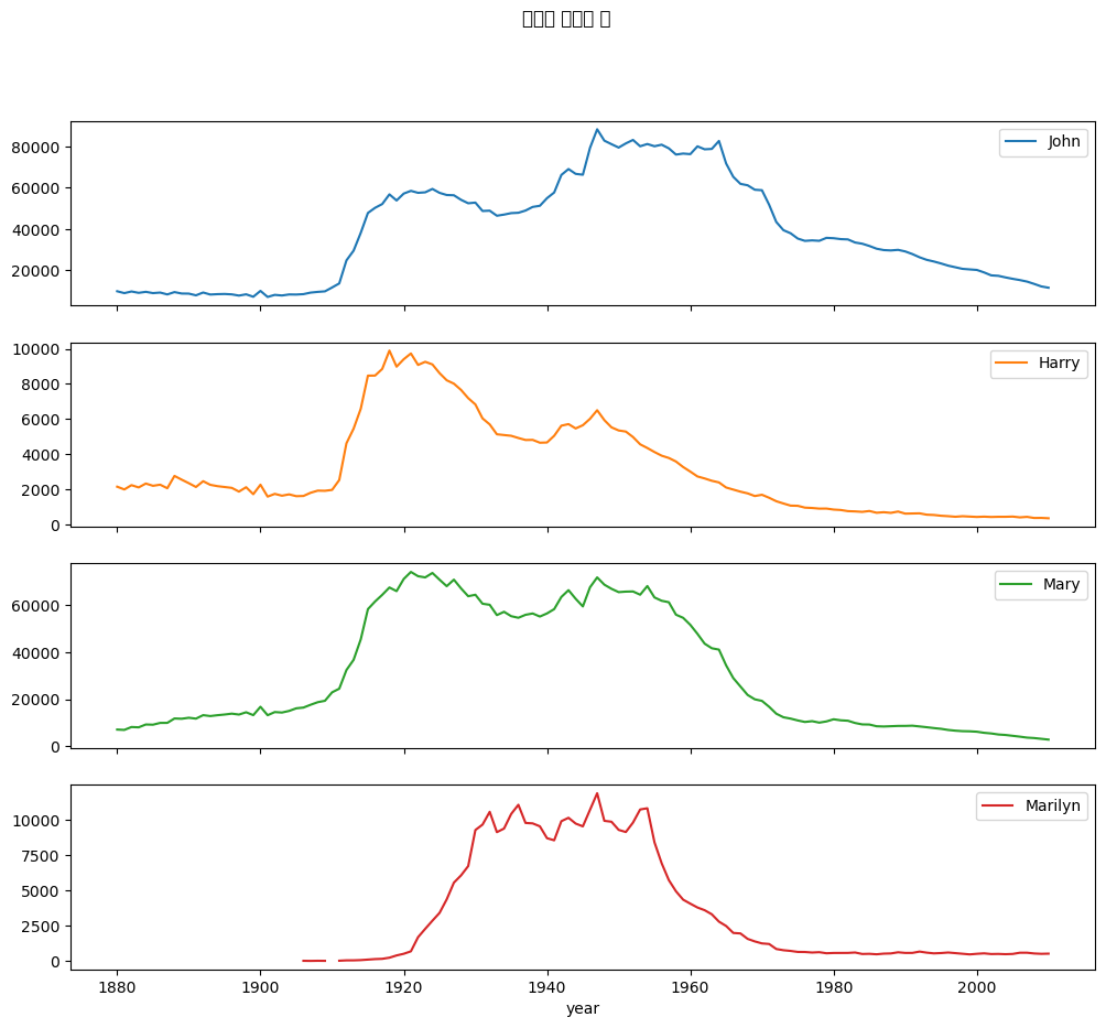
= top1000[top1000["sex" ] == "M" ]= top1000[top1000["sex" ] == "F" ]
= top1000.pivot_table("births" , index= "year" ,= "name" ,= sum )
= total_births[["John" , "Harry" , "Mary" , "Marilyn" ]]= True , figsize= (12 , 10 ),= "연도별 출생아 수" )
<class 'pandas.core.frame.DataFrame'>
Index: 131 entries, 1880 to 2010
Columns: 6868 entries, Aaden to Zuri
dtypes: float64(6868)
memory usage: 6.9 MB
array([<Axes: xlabel='year'>, <Axes: xlabel='year'>,
       <Axes: xlabel='year'>, <Axes: xlabel='year'>], dtype=object)
<Figure size 1000x600 with 0 Axes>
<Figure size 1000x600 with 0 Axes>
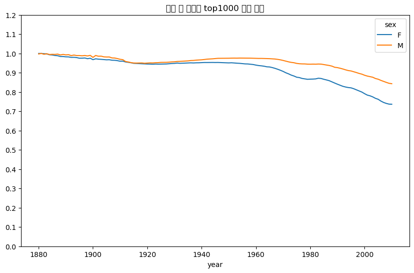
= top1000.pivot_table("prop" , index= "year" ,= "sex" , aggfunc= sum )= "연도 및 성별별 top1000 비중 합계" ,= np.linspace(0 , 1.2 , 13 ))
= boys[boys["year" ] == 2010 ]
260877
Jacob
M
21875
2010
0.011523
260878
Ethan
M
17866
2010
0.009411
260879
Michael
M
17133
2010
0.009025
260880
Jayden
M
17030
2010
0.008971
260881
William
M
16870
2010
0.008887
...
...
...
...
...
...
261872
Camilo
M
194
2010
0.000102
261873
Destin
M
194
2010
0.000102
261874
Jaquan
M
194
2010
0.000102
261875
Jaydan
M
194
2010
0.000102
261876
Maxton
M
193
2010
0.000102
1000 rows × 5 columns
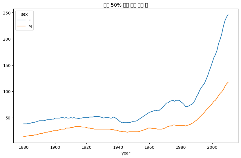
= df["prop" ].sort_values(ascending= False ).cumsum()10 ]0.5 )
= boys[boys.year == 1900 ]= df.sort_values("prop" , ascending= False ).prop.cumsum()0.5 ) + 1
def get_quantile_count(group, q= 0.5 ):= group.sort_values("prop" , ascending= False )return group.prop.cumsum().searchsorted(q) + 1 = top1000.groupby(["year" , "sex" ]).apply (get_quantile_count)= diversity.unstack()
<Figure size 1000x600 with 0 Axes>
= "상위 50% 함유 인기 이름 수" )
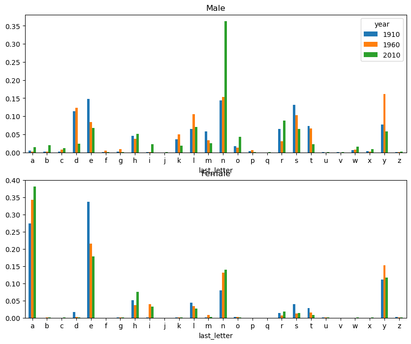
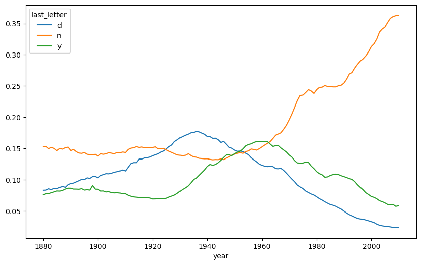
def get_last_letter(x):return x[- 1 ]= names["name" ].map (get_last_letter)= "last_letter" = names.pivot_table("births" , index= last_letters,= ["sex" , "year" ], aggfunc= sum )
= table.reindex(columns= [1910 , 1960 , 2010 ], level= "year" )
year
1910
1960
2010
1910
1960
2010
a
108376.0
691247.0
670605.0
977.0
5204.0
28438.0
b
NaN
694.0
450.0
411.0
3912.0
38859.0
c
5.0
49.0
946.0
482.0
15476.0
23125.0
d
6750.0
3729.0
2607.0
22111.0
262112.0
44398.0
e
133569.0
435013.0
313833.0
28655.0
178823.0
129012.0
sum ()= subtable / subtable.sum ()
year
1910
1960
2010
1910
1960
2010
a
0.273390
0.341853
0.381240
0.005031
0.002440
0.014980
b
NaN
0.000343
0.000256
0.002116
0.001834
0.020470
c
0.000013
0.000024
0.000538
0.002482
0.007257
0.012181
d
0.017028
0.001844
0.001482
0.113858
0.122908
0.023387
e
0.336941
0.215133
0.178415
0.147556
0.083853
0.067959
...
...
...
...
...
...
...
v
NaN
0.000060
0.000117
0.000113
0.000037
0.001434
w
0.000020
0.000031
0.001182
0.006329
0.007711
0.016148
x
0.000015
0.000037
0.000727
0.003965
0.001851
0.008614
y
0.110972
0.152569
0.116828
0.077349
0.160987
0.058168
z
0.002439
0.000659
0.000704
0.000170
0.000184
0.001831
26 rows × 6 columns
import matplotlib.pyplot as plt= plt.subplots(2 , 1 , figsize= (10 , 8 ))"M" ].plot(kind= "bar" , rot= 0 , ax= axes[0 ], title= "Male" )"F" ].plot(kind= "bar" , rot= 0 , ax= axes[1 ], title= "Female" ,= False )
= 0.25 )
<Figure size 1000x600 with 0 Axes>
= table / table.sum ()= letter_prop.loc[["d" , "n" , "y" ], "M" ].T
year
1880
0.083055
0.153213
0.075760
1881
0.083247
0.153214
0.077451
1882
0.085340
0.149560
0.077537
1883
0.084066
0.151646
0.079144
1884
0.086120
0.149915
0.080405
<Figure size 1000x600 with 0 Axes>
= pd.Series(top1000["name" ].unique())= all_names[all_names.str .contains("Lesl" )]
632     Leslie
2294    Lesley
4262    Leslee
4728     Lesli
6103     Lesly
dtype: object
= top1000[top1000["name" ].isin(lesley_like)]"name" )["births" ].sum ()
name
Leslee      1082
Lesley     35022
Lesli        929
Leslie    370429
Lesly      10067
Name: births, dtype: int64
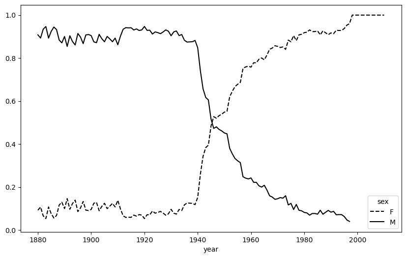
= filtered.pivot_table("births" , index= "year" ,= "sex" , aggfunc= "sum" )= table.div(table.sum (axis= "columns" ), axis= "index" )
year
2006
1.0
NaN
2007
1.0
NaN
2008
1.0
NaN
2009
1.0
NaN
2010
1.0
NaN
<Figure size 1000x600 with 0 Axes>
= {"M" : "k-" , "F" : "k--" })
import json= json.load(open ("datasets/usda_food/database.json" ))len (db)
0 ].keys()0 ]["nutrients" ][0 ]= pd.DataFrame(db[0 ]["nutrients" ])7 )
0
25.18
g
Protein
Composition
1
29.20
g
Total lipid (fat)
Composition
2
3.06
g
Carbohydrate, by difference
Composition
3
3.28
g
Ash
Other
4
376.00
kcal
Energy
Energy
5
39.28
g
Water
Composition
6
1573.00
kJ
Energy
Energy
= ["description" , "group" , "id" , "manufacturer" ]= pd.DataFrame(db, columns= info_keys)
<class 'pandas.core.frame.DataFrame'>
RangeIndex: 6636 entries, 0 to 6635
Data columns (total 4 columns):
 #   Column        Non-Null Count  Dtype
---  ------        --------------  -----
 0   description   6636 non-null   object
 1   group         6636 non-null   object
 2   id            6636 non-null   int64
 3   manufacturer  5195 non-null   object
dtypes: int64(1), object(3)
memory usage: 207.5+ KB
"group" ])[:10 ]
group
Vegetables and Vegetable Products    812
Beef Products                        618
Baked Products                       496
Breakfast Cereals                    403
Legumes and Legume Products          365
Fast Foods                           365
Lamb, Veal, and Game Products        345
Sweets                               341
Fruits and Fruit Juices              328
Pork Products                        328
Name: count, dtype: int64
= []for rec in db:= pd.DataFrame(rec["nutrients" ])"id" ] = rec["id" ]= pd.concat(nutrients, ignore_index= True )
0
25.180
g
Protein
Composition
1008
1
29.200
g
Total lipid (fat)
Composition
1008
2
3.060
g
Carbohydrate, by difference
Composition
1008
3
3.280
g
Ash
Other
1008
4
376.000
kcal
Energy
Energy
1008
...
...
...
...
...
...
389350
0.000
mcg
Vitamin B-12, added
Vitamins
43546
389351
0.000
mg
Cholesterol
Other
43546
389352
0.072
g
Fatty acids, total saturated
Other
43546
389353
0.028
g
Fatty acids, total monounsaturated
Other
43546
389354
0.041
g
Fatty acids, total polyunsaturated
Other
43546
389355 rows × 5 columns
sum () # number of duplicates = nutrients.drop_duplicates()
= {"description" : "food" ,"group" : "fgroup" }= info.rename(columns= col_mapping, copy= False )= {"description" : "nutrient" ,"group" : "nutgroup" }= nutrients.rename(columns= col_mapping, copy= False )
<class 'pandas.core.frame.DataFrame'>
RangeIndex: 6636 entries, 0 to 6635
Data columns (total 4 columns):
 #   Column        Non-Null Count  Dtype
---  ------        --------------  -----
 0   food          6636 non-null   object
 1   fgroup        6636 non-null   object
 2   id            6636 non-null   int64
 3   manufacturer  5195 non-null   object
dtypes: int64(1), object(3)
memory usage: 207.5+ KB
0
25.180
g
Protein
Composition
1008
1
29.200
g
Total lipid (fat)
Composition
1008
2
3.060
g
Carbohydrate, by difference
Composition
1008
3
3.280
g
Ash
Other
1008
4
376.000
kcal
Energy
Energy
1008
...
...
...
...
...
...
389350
0.000
mcg
Vitamin B-12, added
Vitamins
43546
389351
0.000
mg
Cholesterol
Other
43546
389352
0.072
g
Fatty acids, total saturated
Other
43546
389353
0.028
g
Fatty acids, total monounsaturated
Other
43546
389354
0.041
g
Fatty acids, total polyunsaturated
Other
43546
375176 rows × 5 columns
= pd.merge(nutrients, info, on= "id" )30000 ]
<class 'pandas.core.frame.DataFrame'>
RangeIndex: 375176 entries, 0 to 375175
Data columns (total 8 columns):
 #   Column        Non-Null Count   Dtype
---  ------        --------------   -----
 0   value         375176 non-null  float64
 1   units         375176 non-null  object
 2   nutrient      375176 non-null  object
 3   nutgroup      375176 non-null  object
 4   id            375176 non-null  int64
 5   food          375176 non-null  object
 6   fgroup        375176 non-null  object
 7   manufacturer  293054 non-null  object
dtypes: float64(1), int64(1), object(6)
memory usage: 22.9+ MB
value                                             0.04
units                                                g
nutrient                                       Glycine
nutgroup                                   Amino Acids
id                                                6158
food            Soup, tomato bisque, canned, condensed
fgroup                      Soups, Sauces, and Gravies
manufacturer
Name: 30000, dtype: object
<Figure size 1000x600 with 0 Axes>
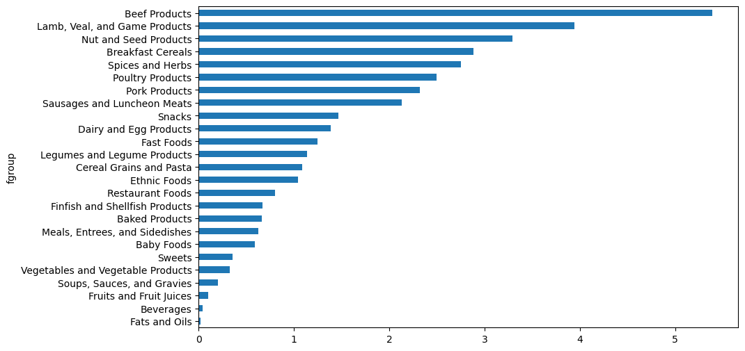
= ndata.groupby(["nutrient" , "fgroup" ])["value" ].quantile(0.5 )"Zinc, Zn" ].sort_values().plot(kind= "barh" )
= ndata.groupby(["nutgroup" , "nutrient" ])def get_maximum(x):return x.loc[x.value.idxmax()]= by_nutrient.apply (get_maximum)[["value" , "food" ]]# make the food a little smaller "food" ] = max_foods["food" ].str [:50 ]
"Amino Acids" ]["food" ]
nutrient
Alanine                            Gelatins, dry powder, unsweetened
Arginine                                Seeds, sesame flour, low-fat
Aspartic acid                                    Soy protein isolate
Cystine                 Seeds, cottonseed flour, low fat (glandless)
Glutamic acid                                    Soy protein isolate
Glycine                            Gelatins, dry powder, unsweetened
Histidine                 Whale, beluga, meat, dried (Alaska Native)
Hydroxyproline    KENTUCKY FRIED CHICKEN, Fried Chicken, ORIGINAL RE
Isoleucine        Soy protein isolate, PROTEIN TECHNOLOGIES INTERNAT
Leucine           Soy protein isolate, PROTEIN TECHNOLOGIES INTERNAT
Lysine            Seal, bearded (Oogruk), meat, dried (Alaska Native
Methionine                     Fish, cod, Atlantic, dried and salted
Phenylalanine     Soy protein isolate, PROTEIN TECHNOLOGIES INTERNAT
Proline                            Gelatins, dry powder, unsweetened
Serine            Soy protein isolate, PROTEIN TECHNOLOGIES INTERNAT
Threonine         Soy protein isolate, PROTEIN TECHNOLOGIES INTERNAT
Tryptophan          Sea lion, Steller, meat with fat (Alaska Native)
Tyrosine          Soy protein isolate, PROTEIN TECHNOLOGIES INTERNAT
Valine            Soy protein isolate, PROTEIN TECHNOLOGIES INTERNAT
Name: food, dtype: object
= pd.read_csv("datasets/fec/P00000001-ALL.csv" , low_memory= False )
<class 'pandas.core.frame.DataFrame'>
RangeIndex: 1001731 entries, 0 to 1001730
Data columns (total 16 columns):
 #   Column             Non-Null Count    Dtype
---  ------             --------------    -----
 0   cmte_id            1001731 non-null  object
 1   cand_id            1001731 non-null  object
 2   cand_nm            1001731 non-null  object
 3   contbr_nm          1001731 non-null  object
 4   contbr_city        1001712 non-null  object
 5   contbr_st          1001727 non-null  object
 6   contbr_zip         1001620 non-null  object
 7   contbr_employer    988002 non-null   object
 8   contbr_occupation  993301 non-null   object
 9   contb_receipt_amt  1001731 non-null  float64
 10  contb_receipt_dt   1001731 non-null  object
 11  receipt_desc       14166 non-null    object
 12  memo_cd            92482 non-null    object
 13  memo_text          97770 non-null    object
 14  form_tp            1001731 non-null  object
 15  file_num           1001731 non-null  int64
dtypes: float64(1), int64(1), object(14)
memory usage: 122.3+ MB
cmte_id                             C00431445
cand_id                             P80003338
cand_nm                         Obama, Barack
contbr_nm                         ELLMAN, IRA
contbr_city                             TEMPE
contbr_st                                  AZ
contbr_zip                          852816719
contbr_employer      ARIZONA STATE UNIVERSITY
contbr_occupation                   PROFESSOR
contb_receipt_amt                        50.0
contb_receipt_dt                    01-DEC-11
receipt_desc                              NaN
memo_cd                                   NaN
memo_text                                 NaN
form_tp                                 SA17A
file_num                               772372
Name: 123456, dtype: object
MovieLens 데이터셋
영화 평점 데이터를 활용하여 분석을 진행합니다.
= fec["cand_nm" ].unique()2 ]
= {"Bachmann, Michelle" : "Republican" ,"Cain, Herman" : "Republican" ,"Gingrich, Newt" : "Republican" ,"Huntsman, Jon" : "Republican" ,"Johnson, Gary Earl" : "Republican" ,"McCotter, Thaddeus G" : "Republican" ,"Obama, Barack" : "Democrat" ,"Paul, Ron" : "Republican" ,"Pawlenty, Timothy" : "Republican" ,"Perry, Rick" : "Republican" ,"Roemer, Charles E. 'Buddy' III" : "Republican" ,"Romney, Mitt" : "Republican" ,"Santorum, Rick" : "Republican" }
"cand_nm" ][123456 :123461 ]"cand_nm" ][123456 :123461 ].map (parties)# Add it as a column "party" ] = fec["cand_nm" ].map (parties)"party" ].value_counts()
party
Democrat      593746
Republican    407985
Name: count, dtype: int64
"contb_receipt_amt" ] > 0 ).value_counts()
contb_receipt_amt
True     991475
False     10256
Name: count, dtype: int64
= fec[fec["contb_receipt_amt" ] > 0 ]
= fec[fec["cand_nm" ].isin(["Obama, Barack" , "Romney, Mitt" ])]
"contbr_occupation" ].value_counts()[:10 ]
contbr_occupation
RETIRED                                   233990
INFORMATION REQUESTED                      35107
ATTORNEY                                   34286
HOMEMAKER                                  29931
PHYSICIAN                                  23432
INFORMATION REQUESTED PER BEST EFFORTS     21138
ENGINEER                                   14334
TEACHER                                    13990
CONSULTANT                                 13273
PROFESSOR                                  12555
Name: count, dtype: int64
= {"INFORMATION REQUESTED PER BEST EFFORTS" : "NOT PROVIDED" ,"INFORMATION REQUESTED" : "NOT PROVIDED" ,"INFORMATION REQUESTED (BEST EFFORTS)" : "NOT PROVIDED" ,"C.E.O." : "CEO" def get_occ(x):# If no mapping provided, return x return occ_mapping.get(x, x)"contbr_occupation" ] = fec["contbr_occupation" ].map (get_occ)
= {"INFORMATION REQUESTED PER BEST EFFORTS" : "NOT PROVIDED" ,"INFORMATION REQUESTED" : "NOT PROVIDED" ,"SELF" : "SELF-EMPLOYED" ,"SELF EMPLOYED" : "SELF-EMPLOYED" ,def get_emp(x):# If no mapping provided, return x return emp_mapping.get(x, x)"contbr_employer" ] = fec["contbr_employer" ].map (get_emp)
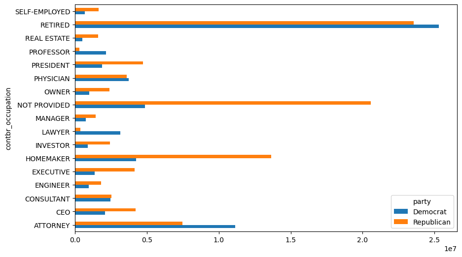
= fec.pivot_table("contb_receipt_amt" ,= "contbr_occupation" ,= "party" , aggfunc= "sum" )= by_occupation[by_occupation.sum (axis= "columns" ) > 2000000 ]
contbr_occupation
ATTORNEY
11141982.97
7477194.43
CEO
2074974.79
4211040.52
CONSULTANT
2459912.71
2544725.45
ENGINEER
951525.55
1818373.70
EXECUTIVE
1355161.05
4138850.09
HOMEMAKER
4248875.80
13634275.78
INVESTOR
884133.00
2431768.92
LAWYER
3160478.87
391224.32
MANAGER
762883.22
1444532.37
NOT PROVIDED
4866973.96
20565473.01
OWNER
1001567.36
2408286.92
PHYSICIAN
3735124.94
3594320.24
PRESIDENT
1878509.95
4720923.76
PROFESSOR
2165071.08
296702.73
REAL ESTATE
528902.09
1625902.25
RETIRED
25305116.38
23561244.49
SELF-EMPLOYED
672393.40
1640252.54
<Figure size 1000x600 with 0 Axes>
<Figure size 1000x600 with 0 Axes>
= "barh" )
def get_top_amounts(group, key, n= 5 ):= group.groupby(key)["contb_receipt_amt" ].sum ()return totals.nlargest(n)
= fec_mrbo.groupby("cand_nm" )apply (get_top_amounts, "contbr_occupation" , n= 7 )apply (get_top_amounts, "contbr_employer" , n= 10 )
cand_nm        contbr_employer
Obama, Barack  RETIRED                                   22694358.85
               SELF-EMPLOYED                             17080985.96
               NOT EMPLOYED                               8586308.70
               INFORMATION REQUESTED                      5053480.37
               HOMEMAKER                                  2605408.54
               SELF                                       1076531.20
               SELF EMPLOYED                               469290.00
               STUDENT                                     318831.45
               VOLUNTEER                                   257104.00
               MICROSOFT                                   215585.36
Romney, Mitt   INFORMATION REQUESTED PER BEST EFFORTS    12059527.24
               RETIRED                                   11506225.71
               HOMEMAKER                                  8147196.22
               SELF-EMPLOYED                              7409860.98
               STUDENT                                     496490.94
               CREDIT SUISSE                               281150.00
               MORGAN STANLEY                              267266.00
               GOLDMAN SACH & CO.                          238250.00
               BARCLAYS CAPITAL                            162750.00
               H.I.G. CAPITAL                              139500.00
Name: contb_receipt_amt, dtype: float64
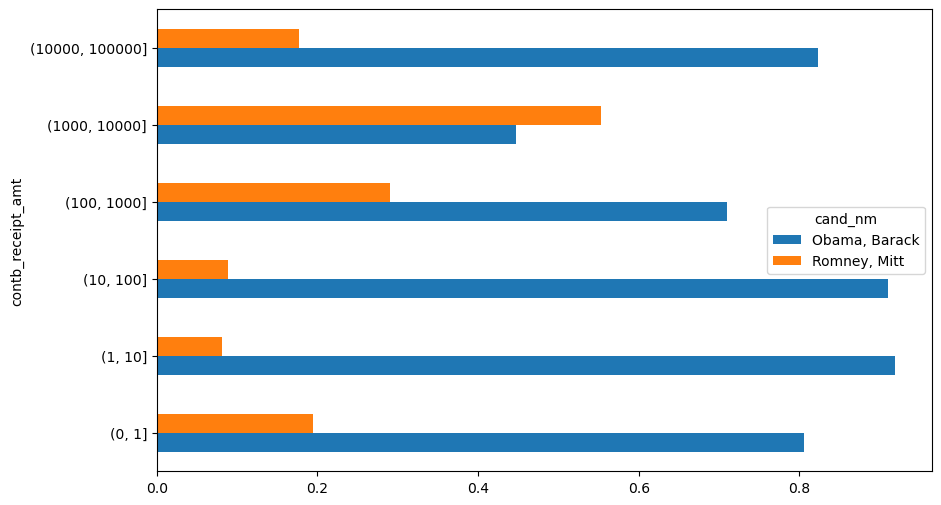
= np.array([0 , 1 , 10 , 100 , 1000 , 10000 ,100_000 , 1_000_000 , 10_000_000 ])= pd.cut(fec_mrbo["contb_receipt_amt" ], bins)
411         (10, 100]
412       (100, 1000]
413       (100, 1000]
414         (10, 100]
415         (10, 100]
             ...
701381      (10, 100]
701382    (100, 1000]
701383        (1, 10]
701384      (10, 100]
701385    (100, 1000]
Name: contb_receipt_amt, Length: 694282, dtype: category
Categories (8, interval[int64, right]): [(0, 1] < (1, 10] < (10, 100] < (100, 1000] < (1000, 10000] < (10000, 100000] < (100000, 1000000] < (1000000, 10000000]]
= fec_mrbo.groupby(["cand_nm" , labels])= 0 )
contb_receipt_amt
(0, 1]
493
77
(1, 10]
40070
3681
(10, 100]
372280
31853
(100, 1000]
153991
43357
(1000, 10000]
22284
26186
(10000, 100000]
2
1
(100000, 1000000]
3
0
(1000000, 10000000]
4
0
<Figure size 1000x600 with 0 Axes>
<Figure size 1000x600 with 0 Axes>
= grouped["contb_receipt_amt" ].sum ().unstack(level= 0 )= bucket_sums.div(bucket_sums.sum (axis= "columns" ),= "index" )- 2 ].plot(kind= "barh" )
= fec_mrbo.groupby(["cand_nm" , "contbr_st" ])= grouped["contb_receipt_amt" ].sum ().unstack(level= 0 ).fillna(0 )= totals[totals.sum (axis= "columns" ) > 100000 ]10 )
contbr_st
AK
281840.15
86204.24
AL
543123.48
527303.51
AR
359247.28
105556.00
AZ
1506476.98
1888436.23
CA
23824984.24
11237636.60
CO
2132429.49
1506714.12
CT
2068291.26
3499475.45
DC
4373538.80
1025137.50
DE
336669.14
82712.00
FL
7318178.58
8338458.81
= totals.div(totals.sum (axis= "columns" ), axis= "index" )10 )
contbr_st
AK
0.765778
0.234222
AL
0.507390
0.492610
AR
0.772902
0.227098
AZ
0.443745
0.556255
CA
0.679498
0.320502
CO
0.585970
0.414030
CT
0.371476
0.628524
DC
0.810113
0.189887
DE
0.802776
0.197224
FL
0.467417
0.532583