import warnings
warnings.filterwarnings('ignore')

import numpy as np
import pandas as pd
np.random.seed(12345)
import matplotlib.pyplot as plt
plt.rc("figure", figsize=(10, 6))
PREVIOUS_MAX_ROWS = pd.options.display.max_rows
pd.options.display.max_columns = 20
pd.options.display.max_rows = 20
pd.options.display.max_colwidth = 80
np.set_printoptions(precision=4, suppress=True)
import matplotlib.pyplot as plt
# Matplotlib 한글 폰트 설정 (macOS용)
plt.rc('font', family='AppleGothic')
plt.rc('axes', unicode_minus=False)10 11장: 시계열
시간의 흐름에 따른 데이터를 분석하기 위한 시계열 특화 기능을 학습합니다.
import numpy as np
import pandas as pd
10.1 날짜, 시간 자료형, 도구
파이썬 내장 datetime 라이브러리와 pandas의 시간 도구들을 비교합니다.
10.2 날짜와 시간 시스템
파이썬의 표준 시간 도구와 pandas의 차이점을 인지합니다.
from datetime import datetime
now = datetime.now()
now
now.year, now.month, now.day
(2026, 2, 26)delta = datetime(2011, 1, 7) - datetime(2008, 6, 24, 8, 15)
delta
delta.days
delta.seconds56700from datetime import timedelta
start = datetime(2011, 1, 7)
start + timedelta(12)
start - 2 * timedelta(12)datetime.datetime(2010, 12, 14, 0, 0)stamp = datetime(2011, 1, 3)
str(stamp)
stamp.strftime("%Y-%m-%d")'2011-01-03'value = "2011-01-03"
datetime.strptime(value, "%Y-%m-%d")
datestrs = ["7/6/2011", "8/6/2011"]
[datetime.strptime(x, "%m/%d/%Y") for x in datestrs][datetime.datetime(2011, 7, 6, 0, 0), datetime.datetime(2011, 8, 6, 0, 0)]datestrs = ["2011-07-06 12:00:00", "2011-08-06 00:00:00"]
pd.to_datetime(datestrs)DatetimeIndex(['2011-07-06 12:00:00', '2011-08-06 00:00:00'], dtype='datetime64[ns]', freq=None)idx = pd.to_datetime(datestrs + [None])
idx
idx[2]
pd.isna(idx)array([False, False, True])10.3 시계열 기초
날짜를 색인으로 사용하는 시계열 객체의 생성과 활용을 배웁니다.
dates = [datetime(2011, 1, 2), datetime(2011, 1, 5),
         datetime(2011, 1, 7), datetime(2011, 1, 8),
         datetime(2011, 1, 10), datetime(2011, 1, 12)]
ts = pd.Series(np.random.standard_normal(6), index=dates)
ts
2011-01-02 -0.204708
2011-01-05 0.478943
2011-01-07 -0.519439
2011-01-08 -0.555730
2011-01-10 1.965781
2011-01-12 1.393406
dtype: float6410.4 시계열 기초
시간을 색인으로 사용하는 Series와 DataFrame을 다루는 방법을 알아봅니다.
ts.indexDatetimeIndex(['2011-01-02', '2011-01-05', '2011-01-07', '2011-01-08',
'2011-01-10', '2011-01-12'],
dtype='datetime64[ns]', freq=None)ts + ts[::2]2011-01-02 -0.409415
2011-01-05 NaN
2011-01-07 -1.038877
2011-01-08 NaN
2011-01-10 3.931561
2011-01-12 NaN
dtype: float64ts.index.dtypedtype('<M8[ns]')stamp = ts.index[0]
stampTimestamp('2011-01-02 00:00:00')stamp = ts.index[2]
ts[stamp]-0.5194387150567381ts["2011-01-10"]1.9657805725027142longer_ts = pd.Series(np.random.standard_normal(1000),
index=pd.date_range("2000-01-01", periods=1000))
longer_ts
longer_ts["2001"]2001-01-01 1.599534
2001-01-02 0.474071
2001-01-03 0.151326
2001-01-04 -0.542173
2001-01-05 -0.475496
...
2001-12-27 0.057874
2001-12-28 -0.433739
2001-12-29 0.092698
2001-12-30 -1.397820
2001-12-31 1.457823
Freq: D, Length: 365, dtype: float64longer_ts["2001-05"]2001-05-01 -0.622547
2001-05-02 0.936289
2001-05-03 0.750018
2001-05-04 -0.056715
2001-05-05 2.300675
...
2001-05-27 0.235477
2001-05-28 0.111835
2001-05-29 -1.251504
2001-05-30 -2.949343
2001-05-31 0.634634
Freq: D, Length: 31, dtype: float64ts[datetime(2011, 1, 7):]
ts[datetime(2011, 1, 7):datetime(2011, 1, 10)]2011-01-07 -0.519439
2011-01-08 -0.555730
2011-01-10 1.965781
dtype: float64ts
ts["2011-01-06":"2011-01-11"]2011-01-07 -0.519439
2011-01-08 -0.555730
2011-01-10 1.965781
dtype: float64ts.truncate(after="2011-01-09")2011-01-02 -0.204708
2011-01-05 0.478943
2011-01-07 -0.519439
2011-01-08 -0.555730
dtype: float64dates = pd.date_range("2000-01-01", periods=100, freq="W-WED")
long_df = pd.DataFrame(np.random.standard_normal((100, 4)),
index=dates,
columns=["Colorado", "Texas",
"New York", "Ohio"])
long_df.loc["2001-05"]| Colorado | Texas | New York | Ohio | |
|---|---|---|---|---|
| 2001-05-02 | -0.006045 | 0.490094 | -0.277186 | -0.707213 |
| 2001-05-09 | -0.560107 | 2.735527 | 0.927335 | 1.513906 |
| 2001-05-16 | 0.538600 | 1.273768 | 0.667876 | -0.969206 |
| 2001-05-23 | 1.676091 | -0.817649 | 0.050188 | 1.951312 |
| 2001-05-30 | 3.260383 | 0.963301 | 1.201206 | -1.852001 |
dates = pd.DatetimeIndex(["2000-01-01", "2000-01-02", "2000-01-02",
                          "2000-01-02", "2000-01-03"])
dup_ts = pd.Series(np.arange(5), index=dates)
dup_ts
2000-01-01 0
2000-01-02 1
2000-01-02 2
2000-01-02 3
2000-01-03 4
dtype: int64dup_ts.index.is_uniqueFalsedup_ts["2000-01-03"] # not duplicated
dup_ts["2000-01-02"] # duplicated2000-01-02 1
2000-01-02 2
2000-01-02 3
dtype: int64grouped = dup_ts.groupby(level=0)
grouped.mean()
grouped.count()2000-01-01 1
2000-01-02 3
2000-01-03 1
dtype: int64ts
resampler = ts.resample("D")
resampler<pandas.core.resample.DatetimeIndexResampler object at 0x15506a910>index = pd.date_range("2012-04-01", "2012-06-01")
indexDatetimeIndex(['2012-04-01', '2012-04-02', '2012-04-03', '2012-04-04',
'2012-04-05', '2012-04-06', '2012-04-07', '2012-04-08',
'2012-04-09', '2012-04-10', '2012-04-11', '2012-04-12',
'2012-04-13', '2012-04-14', '2012-04-15', '2012-04-16',
'2012-04-17', '2012-04-18', '2012-04-19', '2012-04-20',
'2012-04-21', '2012-04-22', '2012-04-23', '2012-04-24',
'2012-04-25', '2012-04-26', '2012-04-27', '2012-04-28',
'2012-04-29', '2012-04-30', '2012-05-01', '2012-05-02',
'2012-05-03', '2012-05-04', '2012-05-05', '2012-05-06',
'2012-05-07', '2012-05-08', '2012-05-09', '2012-05-10',
'2012-05-11', '2012-05-12', '2012-05-13', '2012-05-14',
'2012-05-15', '2012-05-16', '2012-05-17', '2012-05-18',
'2012-05-19', '2012-05-20', '2012-05-21', '2012-05-22',
'2012-05-23', '2012-05-24', '2012-05-25', '2012-05-26',
'2012-05-27', '2012-05-28', '2012-05-29', '2012-05-30',
'2012-05-31', '2012-06-01'],
dtype='datetime64[ns]', freq='D')10.5 날짜 범위, 빈도, 이동
빈도를 지정하여 날짜 범위를 생성하거나 데이터를 앞뒤로 밀어내는 방법(shift)을 배웁니다.
pd.date_range(start="2012-04-01", periods=20)
pd.date_range(end="2012-06-01", periods=20)
DatetimeIndex(['2012-05-13', '2012-05-14', '2012-05-15', '2012-05-16',
'2012-05-17', '2012-05-18', '2012-05-19', '2012-05-20',
'2012-05-21', '2012-05-22', '2012-05-23', '2012-05-24',
'2012-05-25', '2012-05-26', '2012-05-27', '2012-05-28',
'2012-05-29', '2012-05-30', '2012-05-31', '2012-06-01'],
dtype='datetime64[ns]', freq='D')pd.date_range("2000-01-01", "2000-12-01", freq="BM")DatetimeIndex(['2000-01-31', '2000-02-29', '2000-03-31', '2000-04-28',
'2000-05-31', '2000-06-30', '2000-07-31', '2000-08-31',
'2000-09-29', '2000-10-31', '2000-11-30'],
dtype='datetime64[ns]', freq='BM')pd.date_range("2012-05-02 12:56:31", periods=5)DatetimeIndex(['2012-05-02 12:56:31', '2012-05-03 12:56:31',
'2012-05-04 12:56:31', '2012-05-05 12:56:31',
'2012-05-06 12:56:31'],
dtype='datetime64[ns]', freq='D')pd.date_range("2012-05-02 12:56:31", periods=5, normalize=True)DatetimeIndex(['2012-05-02', '2012-05-03', '2012-05-04', '2012-05-05',
'2012-05-06'],
dtype='datetime64[ns]', freq='D')from pandas.tseries.offsets import Hour, Minute
hour = Hour()
hour<Hour>four_hours = Hour(4)
four_hours<4 * Hours>pd.date_range("2000-01-01", "2000-01-03 23:59", freq="4H")DatetimeIndex(['2000-01-01 00:00:00', '2000-01-01 04:00:00',
'2000-01-01 08:00:00', '2000-01-01 12:00:00',
'2000-01-01 16:00:00', '2000-01-01 20:00:00',
'2000-01-02 00:00:00', '2000-01-02 04:00:00',
'2000-01-02 08:00:00', '2000-01-02 12:00:00',
'2000-01-02 16:00:00', '2000-01-02 20:00:00',
'2000-01-03 00:00:00', '2000-01-03 04:00:00',
'2000-01-03 08:00:00', '2000-01-03 12:00:00',
'2000-01-03 16:00:00', '2000-01-03 20:00:00'],
dtype='datetime64[ns]', freq='4H')Hour(2) + Minute(30)<150 * Minutes>pd.date_range("2000-01-01", periods=10, freq="1h30min")DatetimeIndex(['2000-01-01 00:00:00', '2000-01-01 01:30:00',
'2000-01-01 03:00:00', '2000-01-01 04:30:00',
'2000-01-01 06:00:00', '2000-01-01 07:30:00',
'2000-01-01 09:00:00', '2000-01-01 10:30:00',
'2000-01-01 12:00:00', '2000-01-01 13:30:00'],
dtype='datetime64[ns]', freq='90T')monthly_dates = pd.date_range("2012-01-01", "2012-09-01", freq="WOM-3FRI")
list(monthly_dates)[Timestamp('2012-01-20 00:00:00'),
Timestamp('2012-02-17 00:00:00'),
Timestamp('2012-03-16 00:00:00'),
Timestamp('2012-04-20 00:00:00'),
Timestamp('2012-05-18 00:00:00'),
Timestamp('2012-06-15 00:00:00'),
Timestamp('2012-07-20 00:00:00'),
Timestamp('2012-08-17 00:00:00')]10.6 데이터 이동과 빈도
시간축을 따라 데이터를 앞뒤로 이동시키는 연산을 수행합니다.
ts = pd.Series(np.random.standard_normal(4),
               index=pd.date_range("2000-01-01", periods=4, freq="M"))
ts
ts.shift(2)
ts.shift(-2)
2000-01-31 -0.117388
2000-02-29 -0.517795
2000-03-31 NaN
2000-04-30 NaN
Freq: M, dtype: float64ts.shift(2, freq="M")2000-03-31 -0.066748
2000-04-30 0.838639
2000-05-31 -0.117388
2000-06-30 -0.517795
Freq: M, dtype: float64ts.shift(3, freq="D")
ts.shift(1, freq="90T")2000-01-31 01:30:00 -0.066748
2000-02-29 01:30:00 0.838639
2000-03-31 01:30:00 -0.117388
2000-04-30 01:30:00 -0.517795
dtype: float64from pandas.tseries.offsets import Day, MonthEnd
now = datetime(2011, 11, 17)
now + 3 * Day()Timestamp('2011-11-20 00:00:00')now + MonthEnd()
now + MonthEnd(2)Timestamp('2011-12-31 00:00:00')offset = MonthEnd()
offset.rollforward(now)
offset.rollback(now)Timestamp('2011-10-31 00:00:00')ts = pd.Series(np.random.standard_normal(20),
index=pd.date_range("2000-01-15", periods=20, freq="4D"))
ts
ts.groupby(MonthEnd().rollforward).mean()2000-01-31 -0.005833
2000-02-29 0.015894
2000-03-31 0.150209
dtype: float64ts.resample("M").mean()2000-01-31 -0.005833
2000-02-29 0.015894
2000-03-31 0.150209
Freq: M, dtype: float64import pytz
pytz.common_timezones[-5:]['US/Eastern', 'US/Hawaii', 'US/Mountain', 'US/Pacific', 'UTC']10.7 시간대 처리
국제화된 데이터를 다루기 위한 시간대(time zone) 변환 작업을 수행합니다.
tz = pytz.timezone("America/New_York")
tz
<DstTzInfo 'America/New_York' LMT-1 day, 19:04:00 STD>dates = pd.date_range("2012-03-09 09:30", periods=6)
ts = pd.Series(np.random.standard_normal(len(dates)), index=dates)
ts2012-03-09 09:30:00 -0.202469
2012-03-10 09:30:00 0.050718
2012-03-11 09:30:00 0.639869
2012-03-12 09:30:00 0.597594
2012-03-13 09:30:00 -0.797246
2012-03-14 09:30:00 0.472879
Freq: D, dtype: float64print(ts.index.tz)Nonepd.date_range("2012-03-09 09:30", periods=10, tz="UTC")DatetimeIndex(['2012-03-09 09:30:00+00:00', '2012-03-10 09:30:00+00:00',
'2012-03-11 09:30:00+00:00', '2012-03-12 09:30:00+00:00',
'2012-03-13 09:30:00+00:00', '2012-03-14 09:30:00+00:00',
'2012-03-15 09:30:00+00:00', '2012-03-16 09:30:00+00:00',
'2012-03-17 09:30:00+00:00', '2012-03-18 09:30:00+00:00'],
dtype='datetime64[ns, UTC]', freq='D')10.8 시간대 처리
글로벌 데이터를 분석할 때 필수적인 시간대 변환 기법을 알아봅니다.
ts
ts_utc = ts.tz_localize("UTC")
ts_utc
ts_utc.index
DatetimeIndex(['2012-03-09 09:30:00+00:00', '2012-03-10 09:30:00+00:00',
'2012-03-11 09:30:00+00:00', '2012-03-12 09:30:00+00:00',
'2012-03-13 09:30:00+00:00', '2012-03-14 09:30:00+00:00'],
dtype='datetime64[ns, UTC]', freq='D')ts_utc.tz_convert("America/New_York")2012-03-09 04:30:00-05:00 -0.202469
2012-03-10 04:30:00-05:00 0.050718
2012-03-11 05:30:00-04:00 0.639869
2012-03-12 05:30:00-04:00 0.597594
2012-03-13 05:30:00-04:00 -0.797246
2012-03-14 05:30:00-04:00 0.472879
Freq: D, dtype: float64ts_eastern = ts.tz_localize("America/New_York")
ts_eastern.tz_convert("UTC")
ts_eastern.tz_convert("Europe/Berlin")2012-03-09 15:30:00+01:00 -0.202469
2012-03-10 15:30:00+01:00 0.050718
2012-03-11 14:30:00+01:00 0.639869
2012-03-12 14:30:00+01:00 0.597594
2012-03-13 14:30:00+01:00 -0.797246
2012-03-14 14:30:00+01:00 0.472879
dtype: float64ts.index.tz_localize("Asia/Shanghai")DatetimeIndex(['2012-03-09 09:30:00+08:00', '2012-03-10 09:30:00+08:00',
'2012-03-11 09:30:00+08:00', '2012-03-12 09:30:00+08:00',
'2012-03-13 09:30:00+08:00', '2012-03-14 09:30:00+08:00'],
dtype='datetime64[ns, Asia/Shanghai]', freq=None)stamp = pd.Timestamp("2011-03-12 04:00")
stamp_utc = stamp.tz_localize("utc")
stamp_utc.tz_convert("America/New_York")Timestamp('2011-03-11 23:00:00-0500', tz='America/New_York')stamp_moscow = pd.Timestamp("2011-03-12 04:00", tz="Europe/Moscow")
stamp_moscowTimestamp('2011-03-12 04:00:00+0300', tz='Europe/Moscow')stamp_utc.value
stamp_utc.tz_convert("America/New_York").value1299902400000000000stamp = pd.Timestamp("2012-03-11 01:30", tz="US/Eastern")
stamp
stamp + Hour()Timestamp('2012-03-11 03:30:00-0400', tz='US/Eastern')stamp = pd.Timestamp("2012-11-04 00:30", tz="US/Eastern")
stamp
stamp + 2 * Hour()Timestamp('2012-11-04 01:30:00-0500', tz='US/Eastern')dates = pd.date_range("2012-03-07 09:30", periods=10, freq="B")
ts = pd.Series(np.random.standard_normal(len(dates)), index=dates)
ts
ts1 = ts[:7].tz_localize("Europe/London")
ts2 = ts1[2:].tz_convert("Europe/Moscow")
result = ts1 + ts2
result.indexDatetimeIndex(['2012-03-07 09:30:00+00:00', '2012-03-08 09:30:00+00:00',
'2012-03-09 09:30:00+00:00', '2012-03-12 09:30:00+00:00',
'2012-03-13 09:30:00+00:00', '2012-03-14 09:30:00+00:00',
'2012-03-15 09:30:00+00:00'],
dtype='datetime64[ns, UTC]', freq=None)p = pd.Period("2011", freq="A-DEC")
pPeriod('2011', 'A-DEC')p + 5
p - 2Period('2009', 'A-DEC')pd.Period("2014", freq="A-DEC") - p<3 * YearEnds: month=12>periods = pd.period_range("2000-01-01", "2000-06-30", freq="M")
periodsPeriodIndex(['2000-01', '2000-02', '2000-03', '2000-04', '2000-05', '2000-06'], dtype='period[M]')pd.Series(np.random.standard_normal(6), index=periods)2000-01 -0.514551
2000-02 -0.559782
2000-03 -0.783408
2000-04 -1.797685
2000-05 -0.172670
2000-06 0.680215
Freq: M, dtype: float64values = ["2001Q3", "2002Q2", "2003Q1"]
index = pd.PeriodIndex(values, freq="Q-DEC")
indexPeriodIndex(['2001Q3', '2002Q2', '2003Q1'], dtype='period[Q-DEC]')p = pd.Period("2011", freq="A-DEC")
p
p.asfreq("M", how="start")
p.asfreq("M", how="end")
p.asfreq("M")Period('2011-12', 'M')p = pd.Period("2011", freq="A-JUN")
p
p.asfreq("M", how="start")
p.asfreq("M", how="end")Period('2011-06', 'M')p = pd.Period("Aug-2011", "M")
p.asfreq("A-JUN")Period('2012', 'A-JUN')periods = pd.period_range("2006", "2009", freq="A-DEC")
ts = pd.Series(np.random.standard_normal(len(periods)), index=periods)
ts
ts.asfreq("M", how="start")2006-01 1.607578
2007-01 0.200381
2008-01 -0.834068
2009-01 -0.302988
Freq: M, dtype: float64ts.asfreq("B", how="end")2006-12-29 1.607578
2007-12-31 0.200381
2008-12-31 -0.834068
2009-12-31 -0.302988
Freq: B, dtype: float64p = pd.Period("2012Q4", freq="Q-JAN")
pPeriod('2012Q4', 'Q-JAN')p.asfreq("D", how="start")
p.asfreq("D", how="end")Period('2012-01-31', 'D')p4pm = (p.asfreq("B", how="end") - 1).asfreq("T", how="start") + 16 * 60
p4pm
p4pm.to_timestamp()Timestamp('2012-01-30 16:00:00')periods = pd.period_range("2011Q3", "2012Q4", freq="Q-JAN")
ts = pd.Series(np.arange(len(periods)), index=periods)
ts
new_periods = (periods.asfreq("B", "end") - 1).asfreq("H", "start") + 16
ts.index = new_periods.to_timestamp()
ts2010-10-28 16:00:00 0
2011-01-28 16:00:00 1
2011-04-28 16:00:00 2
2011-07-28 16:00:00 3
2011-10-28 16:00:00 4
2012-01-30 16:00:00 5
dtype: int64dates = pd.date_range("2000-01-01", periods=3, freq="M")
ts = pd.Series(np.random.standard_normal(3), index=dates)
ts
pts = ts.to_period()
pts2000-01 1.663261
2000-02 -0.996206
2000-03 1.521760
Freq: M, dtype: float64dates = pd.date_range("2000-01-29", periods=6)
ts2 = pd.Series(np.random.standard_normal(6), index=dates)
ts2
ts2.to_period("M")2000-01 0.244175
2000-01 0.423331
2000-01 -0.654040
2000-02 2.089154
2000-02 -0.060220
2000-02 -0.167933
Freq: M, dtype: float64pts = ts2.to_period()
pts
pts.to_timestamp(how="end")2000-01-29 23:59:59.999999999 0.244175
2000-01-30 23:59:59.999999999 0.423331
2000-01-31 23:59:59.999999999 -0.654040
2000-02-01 23:59:59.999999999 2.089154
2000-02-02 23:59:59.999999999 -0.060220
2000-02-03 23:59:59.999999999 -0.167933
Freq: D, dtype: float64data = pd.read_csv("examples/macrodata.csv")
data.head(5)
data["year"]
data["quarter"]0 1
1 2
2 3
3 4
4 1
..
198 3
199 4
200 1
201 2
202 3
Name: quarter, Length: 203, dtype: int64index = pd.PeriodIndex(year=data["year"], quarter=data["quarter"],
freq="Q-DEC")
index
data.index = index
data["infl"]1959Q1 0.00
1959Q2 2.34
1959Q3 2.74
1959Q4 0.27
1960Q1 2.31
...
2008Q3 -3.16
2008Q4 -8.79
2009Q1 0.94
2009Q2 3.37
2009Q3 3.56
Freq: Q-DEC, Name: infl, Length: 203, dtype: float64dates = pd.date_range("2000-01-01", periods=100)
ts = pd.Series(np.random.standard_normal(len(dates)), index=dates)
ts
ts.resample("M").mean()
ts.resample("M", kind="period").mean()2000-01 -0.165893
2000-02 0.078606
2000-03 0.223811
2000-04 -0.063643
Freq: M, dtype: float64dates = pd.date_range("2000-01-01", periods=12, freq="T")
ts = pd.Series(np.arange(len(dates)), index=dates)
ts2000-01-01 00:00:00 0
2000-01-01 00:01:00 1
2000-01-01 00:02:00 2
2000-01-01 00:03:00 3
2000-01-01 00:04:00 4
2000-01-01 00:05:00 5
2000-01-01 00:06:00 6
2000-01-01 00:07:00 7
2000-01-01 00:08:00 8
2000-01-01 00:09:00 9
2000-01-01 00:10:00 10
2000-01-01 00:11:00 11
Freq: T, dtype: int64ts.resample("5min").sum()2000-01-01 00:00:00 10
2000-01-01 00:05:00 35
2000-01-01 00:10:00 21
Freq: 5T, dtype: int64ts.resample("5min", closed="right").sum()1999-12-31 23:55:00 0
2000-01-01 00:00:00 15
2000-01-01 00:05:00 40
2000-01-01 00:10:00 11
Freq: 5T, dtype: int64ts.resample("5min", closed="right", label="right").sum()2000-01-01 00:00:00 0
2000-01-01 00:05:00 15
2000-01-01 00:10:00 40
2000-01-01 00:15:00 11
Freq: 5T, dtype: int64from pandas.tseries.frequencies import to_offset
result = ts.resample("5min", closed="right", label="right").sum()
result.index = result.index + to_offset("-1s")
result1999-12-31 23:59:59 0
2000-01-01 00:04:59 15
2000-01-01 00:09:59 40
2000-01-01 00:14:59 11
Freq: 5T, dtype: int64ts = pd.Series(np.random.permutation(np.arange(len(dates))), index=dates)
ts.resample("5min").ohlc()| open | high | low | close | |
|---|---|---|---|---|
| 2000-01-01 00:00:00 | 8 | 8 | 1 | 5 |
| 2000-01-01 00:05:00 | 6 | 11 | 2 | 2 |
| 2000-01-01 00:10:00 | 0 | 7 | 0 | 7 |
frame = pd.DataFrame(np.random.standard_normal((2, 4)),
                     index=pd.date_range("2000-01-01", periods=2,
                                         freq="W-WED"),
                     columns=["Colorado", "Texas", "New York", "Ohio"])
frame| Colorado | Texas | New York | Ohio | |
|---|---|---|---|---|
| 2000-01-05 | -0.896431 | 0.927238 | 0.482284 | -0.867130 |
| 2000-01-12 | 0.493841 | -0.155434 | 1.397286 | 1.507055 |
df_daily = frame.resample("D").asfreq()
df_daily| Colorado | Texas | New York | Ohio | |
|---|---|---|---|---|
| 2000-01-05 | -0.896431 | 0.927238 | 0.482284 | -0.867130 |
| 2000-01-06 | NaN | NaN | NaN | NaN |
| 2000-01-07 | NaN | NaN | NaN | NaN |
| 2000-01-08 | NaN | NaN | NaN | NaN |
| 2000-01-09 | NaN | NaN | NaN | NaN |
| 2000-01-10 | NaN | NaN | NaN | NaN |
| 2000-01-11 | NaN | NaN | NaN | NaN |
| 2000-01-12 | 0.493841 | -0.155434 | 1.397286 | 1.507055 |
frame.resample("D").ffill()| Colorado | Texas | New York | Ohio | |
|---|---|---|---|---|
| 2000-01-05 | -0.896431 | 0.927238 | 0.482284 | -0.867130 |
| 2000-01-06 | -0.896431 | 0.927238 | 0.482284 | -0.867130 |
| 2000-01-07 | -0.896431 | 0.927238 | 0.482284 | -0.867130 |
| 2000-01-08 | -0.896431 | 0.927238 | 0.482284 | -0.867130 |
| 2000-01-09 | -0.896431 | 0.927238 | 0.482284 | -0.867130 |
| 2000-01-10 | -0.896431 | 0.927238 | 0.482284 | -0.867130 |
| 2000-01-11 | -0.896431 | 0.927238 | 0.482284 | -0.867130 |
| 2000-01-12 | 0.493841 | -0.155434 | 1.397286 | 1.507055 |
frame.resample("D").ffill(limit=2)| Colorado | Texas | New York | Ohio | |
|---|---|---|---|---|
| 2000-01-05 | -0.896431 | 0.927238 | 0.482284 | -0.867130 |
| 2000-01-06 | -0.896431 | 0.927238 | 0.482284 | -0.867130 |
| 2000-01-07 | -0.896431 | 0.927238 | 0.482284 | -0.867130 |
| 2000-01-08 | NaN | NaN | NaN | NaN |
| 2000-01-09 | NaN | NaN | NaN | NaN |
| 2000-01-10 | NaN | NaN | NaN | NaN |
| 2000-01-11 | NaN | NaN | NaN | NaN |
| 2000-01-12 | 0.493841 | -0.155434 | 1.397286 | 1.507055 |
frame.resample("W-THU").ffill()| Colorado | Texas | New York | Ohio | |
|---|---|---|---|---|
| 2000-01-06 | -0.896431 | 0.927238 | 0.482284 | -0.867130 |
| 2000-01-13 | 0.493841 | -0.155434 | 1.397286 | 1.507055 |
frame = pd.DataFrame(np.random.standard_normal((24, 4)),
                     index=pd.period_range("1-2000", "12-2001",
                                           freq="M"),
                     columns=["Colorado", "Texas", "New York", "Ohio"])
frame.head()
annual_frame = frame.resample("A-DEC").mean()
annual_frame| Colorado | Texas | New York | Ohio | |
|---|---|---|---|---|
| 2000 | 0.487329 | 0.104466 | 0.020495 | -0.273945 |
| 2001 | 0.203125 | 0.162429 | 0.056146 | -0.103794 |
# Q-DEC: Quarterly, year ending in December
annual_frame.resample("Q-DEC").ffill()
annual_frame.resample("Q-DEC", convention="end").asfreq()| Colorado | Texas | New York | Ohio | |
|---|---|---|---|---|
| 2000Q4 | 0.487329 | 0.104466 | 0.020495 | -0.273945 |
| 2001Q1 | NaN | NaN | NaN | NaN |
| 2001Q2 | NaN | NaN | NaN | NaN |
| 2001Q3 | NaN | NaN | NaN | NaN |
| 2001Q4 | 0.203125 | 0.162429 | 0.056146 | -0.103794 |
annual_frame.resample("Q-MAR").ffill()| Colorado | Texas | New York | Ohio | |
|---|---|---|---|---|
| 2000Q4 | 0.487329 | 0.104466 | 0.020495 | -0.273945 |
| 2001Q1 | 0.487329 | 0.104466 | 0.020495 | -0.273945 |
| 2001Q2 | 0.487329 | 0.104466 | 0.020495 | -0.273945 |
| 2001Q3 | 0.487329 | 0.104466 | 0.020495 | -0.273945 |
| 2001Q4 | 0.203125 | 0.162429 | 0.056146 | -0.103794 |
| 2002Q1 | 0.203125 | 0.162429 | 0.056146 | -0.103794 |
| 2002Q2 | 0.203125 | 0.162429 | 0.056146 | -0.103794 |
| 2002Q3 | 0.203125 | 0.162429 | 0.056146 | -0.103794 |
N = 15
times = pd.date_range("2017-05-20 00:00", freq="1min", periods=N)
df = pd.DataFrame({"time": times,
                   "value": np.arange(N)})
df| time | value | |
|---|---|---|
| 0 | 2017-05-20 00:00:00 | 0 |
| 1 | 2017-05-20 00:01:00 | 1 |
| 2 | 2017-05-20 00:02:00 | 2 |
| 3 | 2017-05-20 00:03:00 | 3 |
| 4 | 2017-05-20 00:04:00 | 4 |
| 5 | 2017-05-20 00:05:00 | 5 |
| 6 | 2017-05-20 00:06:00 | 6 |
| 7 | 2017-05-20 00:07:00 | 7 |
| 8 | 2017-05-20 00:08:00 | 8 |
| 9 | 2017-05-20 00:09:00 | 9 |
| 10 | 2017-05-20 00:10:00 | 10 |
| 11 | 2017-05-20 00:11:00 | 11 |
| 12 | 2017-05-20 00:12:00 | 12 |
| 13 | 2017-05-20 00:13:00 | 13 |
| 14 | 2017-05-20 00:14:00 | 14 |
df.set_index("time").resample("5min").count()| value | |
|---|---|
| time | |
| 2017-05-20 00:00:00 | 5 |
| 2017-05-20 00:05:00 | 5 |
| 2017-05-20 00:10:00 | 5 |
df2 = pd.DataFrame({"time": times.repeat(3),
                    "key": np.tile(["a", "b", "c"], N),
                    "value": np.arange(N * 3.)})
df2.head(7)| time | key | value | |
|---|---|---|---|
| 0 | 2017-05-20 00:00:00 | a | 0.0 |
| 1 | 2017-05-20 00:00:00 | b | 1.0 |
| 2 | 2017-05-20 00:00:00 | c | 2.0 |
| 3 | 2017-05-20 00:01:00 | a | 3.0 |
| 4 | 2017-05-20 00:01:00 | b | 4.0 |
| 5 | 2017-05-20 00:01:00 | c | 5.0 |
| 6 | 2017-05-20 00:02:00 | a | 6.0 |
time_key = pd.Grouper(freq="5min")resampled = (df2.set_index("time")
.groupby(["key", time_key])
.sum())
resampled
resampled.reset_index()| key | time | value | |
|---|---|---|---|
| 0 | a | 2017-05-20 00:00:00 | 30.0 |
| 1 | a | 2017-05-20 00:05:00 | 105.0 |
| 2 | a | 2017-05-20 00:10:00 | 180.0 |
| 3 | b | 2017-05-20 00:00:00 | 35.0 |
| 4 | b | 2017-05-20 00:05:00 | 110.0 |
| 5 | b | 2017-05-20 00:10:00 | 185.0 |
| 6 | c | 2017-05-20 00:00:00 | 40.0 |
| 7 | c | 2017-05-20 00:05:00 | 115.0 |
| 8 | c | 2017-05-20 00:10:00 | 190.0 |
close_px_all = pd.read_csv("examples/stock_px.csv",
                           parse_dates=True, index_col=0)
close_px = close_px_all[["AAPL", "MSFT", "XOM"]]
close_px = close_px.resample("B").ffill()close_px["AAPL"].plot()
close_px["AAPL"].rolling(250).mean().plot()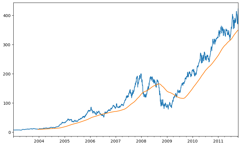
plt.figure()
std250 = close_px["AAPL"].pct_change().rolling(250, min_periods=10).std()
std250[5:12]
std250.plot()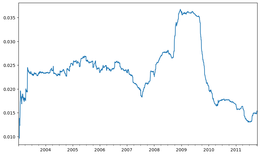
expanding_mean = std250.expanding().mean()plt.figure()<Figure size 1000x600 with 0 Axes><Figure size 1000x600 with 0 Axes>plt.style.use('grayscale')
close_px.rolling(60).mean().plot(logy=True)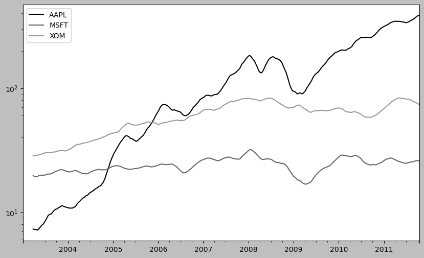
close_px.rolling("20D").mean()| AAPL | MSFT | XOM | |
|---|---|---|---|
| 2003-01-02 | 7.400000 | 21.110000 | 29.220000 |
| 2003-01-03 | 7.425000 | 21.125000 | 29.230000 |
| 2003-01-06 | 7.433333 | 21.256667 | 29.473333 |
| 2003-01-07 | 7.432500 | 21.425000 | 29.342500 |
| 2003-01-08 | 7.402000 | 21.402000 | 29.240000 |
| ... | ... | ... | ... |
| 2011-10-10 | 389.351429 | 25.602143 | 72.527857 |
| 2011-10-11 | 388.505000 | 25.674286 | 72.835000 |
| 2011-10-12 | 388.531429 | 25.810000 | 73.400714 |
| 2011-10-13 | 388.826429 | 25.961429 | 73.905000 |
| 2011-10-14 | 391.038000 | 26.048667 | 74.185333 |
2292 rows × 3 columns
plt.figure()<Figure size 1000x600 with 0 Axes><Figure size 1000x600 with 0 Axes>aapl_px = close_px["AAPL"]["2006":"2007"]
ma30 = aapl_px.rolling(30, min_periods=20).mean()
ewma30 = aapl_px.ewm(span=30).mean()
aapl_px.plot(style="k-", label="Price")
ma30.plot(style="k--", label="Simple Moving Avg")
ewma30.plot(style="k-", label="EW MA")
plt.legend()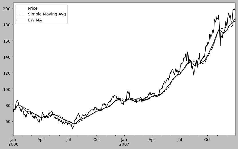
plt.figure()<Figure size 1000x600 with 0 Axes><Figure size 1000x600 with 0 Axes>spx_px = close_px_all["SPX"]
spx_rets = spx_px.pct_change()
returns = close_px.pct_change()corr = returns["AAPL"].rolling(125, min_periods=100).corr(spx_rets)
corr.plot()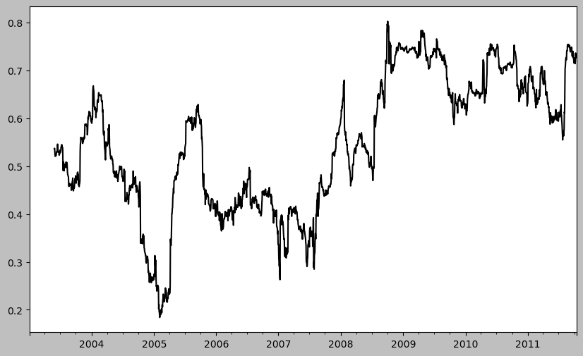
plt.figure()<Figure size 1000x600 with 0 Axes><Figure size 1000x600 with 0 Axes>corr = returns.rolling(125, min_periods=100).corr(spx_rets)
corr.plot()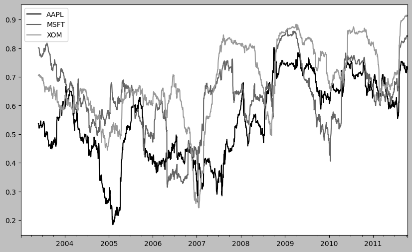
plt.figure()<Figure size 1000x600 with 0 Axes><Figure size 1000x600 with 0 Axes>from scipy.stats import percentileofscore
def score_at_2percent(x):
return percentileofscore(x, 0.02)
result = returns["AAPL"].rolling(250).apply(score_at_2percent)
result.plot()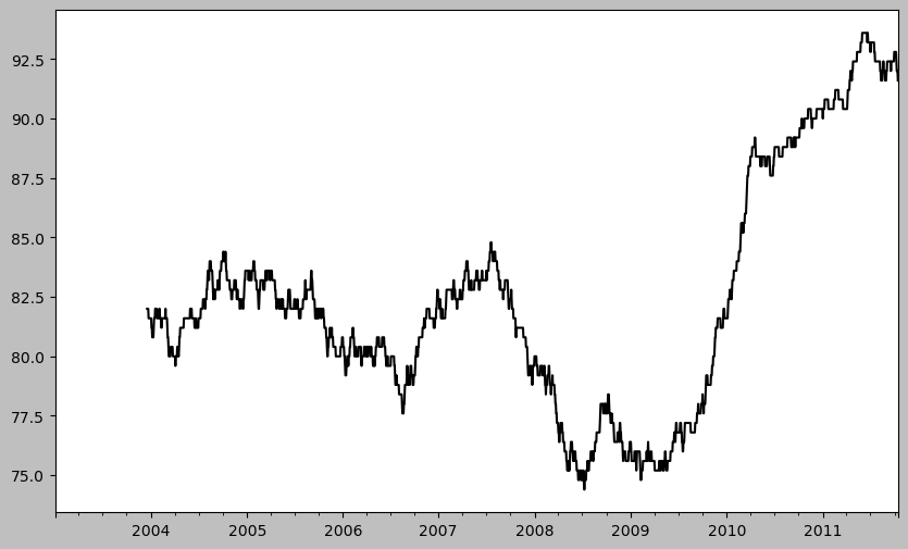
pd.options.display.max_rows = PREVIOUS_MAX_ROWS