10장 - 지역 실험과 스위치백 실험

from toolz.curried import *

import pandas as pd
import numpy as np

import statsmodels.formula.api as smf

from matplotlib import pyplot as plt
from cycler import cycler

color = ["0.0", "0.4", "0.8"]
default_cycler = cycler(color=color)
linestyle = ["-", "--", ":", "-."]
marker = ["o", "v", "d", "p"]

plt.rc("axes", prop_cycle=default_cycler)

from sklearn.base import BaseEstimator, RegressorMixin
from sklearn.utils.validation import check_X_y, check_array, check_is_fitted
import cvxpy as cp


class SyntheticControl(BaseEstimator, RegressorMixin):
    def __init__(self, fit_intercept=False):
        self.fit_intercept = fit_intercept

    def fit(self, y_pre_co, y_pre_tr):
        y_pre_co, y_pre_tr = check_X_y(y_pre_co, y_pre_tr)

        # add intercept
        intercept = np.ones((y_pre_co.shape[0], 1)) * self.fit_intercept
        X = np.concatenate([intercept, y_pre_co], axis=1)
        w = cp.Variable(X.shape[1])

        objective = cp.Minimize(cp.sum_squares(X @ w - y_pre_tr))
        constraints = [cp.sum(w[1:]) == 1, w[1:] >= 0]

        problem = cp.Problem(objective, constraints)

        self.loss_ = problem.solve(eps_abs=1)
        self.w_ = w.value[1:]
        self.intercept_ = w.value[0]

        self.is_fitted_ = True
        return self

    def predict(self, y_co):
        check_is_fitted(self)
        y_co = check_array(y_co)

        return y_co @ self.w_ + self.intercept_

10.1 지역 실험

지역 기반의 실험 설계를 통해 간섭 효과(Interference) 문제를 해결할 수 있습니다.

df = (
    pd.read_csv("../data/online_mkt.csv")
    .astype({"date": "datetime64[ns]"})
    .query("post==0")
)

df.head()

	app_download	population	city	state	date	post	treated
0	3066.0	12396372	sao_paulo	sao_paulo	2022-03-01	0	1
1	2701.0	12396372	sao_paulo	sao_paulo	2022-03-02	0	1
2	1927.0	12396372	sao_paulo	sao_paulo	2022-03-03	0	1
3	1451.0	12396372	sao_paulo	sao_paulo	2022-03-04	0	1
4	1248.0	12396372	sao_paulo	sao_paulo	2022-03-05	0	1

detectable_diff = df["app_download"].mean() * 0.05
sigma_2 = df.groupby("city")["app_download"].mean().var()

np.ceil((sigma_2 * 16) / (detectable_diff) ** 2)

36663.0

10.2 통제집단합성법 설계

pd.set_option("display.max_columns", 6)

df_piv = df.pivot("date", "city", "app_download")

df_piv.head()

city	ananindeua	aparecida_de_goiania	aracaju	...	teresina	uberlandia	vila_velha
date
2022-03-01	11.0	54.0	65.0	...	68.0	29.0	63.0
2022-03-02	5.0	20.0	42.0	...	17.0	29.0	11.0
2022-03-03	2.0	0.0	0.0	...	55.0	30.0	14.0
2022-03-04	0.0	0.0	11.0	...	49.0	35.0	0.0
2022-03-05	5.0	5.0	0.0	...	31.0	6.0	1.0

5 rows × 50 columns

f = (
    df.groupby("city")["population"].first()
    / df.groupby("city")["population"].first().sum()
)

plt.figure(figsize=(12, 3))
plt.bar(f.sort_values().index, f.sort_values().values)
plt.title("Size of each city as a proportional of the market (f vector)")
plt.xticks(rotation=90, fontsize=14);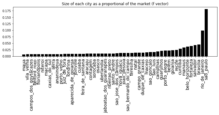

10.2.1 무작위로 실험군 선택하기

y_avg = df_piv.dot(f)
geos = list(df_piv.columns)
n_tr = 5

np.random.seed(42)
rand_geos = np.random.choice(geos, n_tr, replace=False)
rand_geos

array(['manaus', 'recife', 'sao_bernardo_do_campo', 'salvador', 'aracaju'],
      dtype='<U23')

def get_sc(geos, df_sc, y_mean_pre):
    model = SyntheticControl(fit_intercept=True)
    model.fit(df_sc[geos], y_mean_pre)

    selected_geos = geos[np.abs(model.w_) > 1e-5]

    return {"geos": selected_geos, "loss": model.loss_}


get_sc(rand_geos, df_piv, y_avg)

{'geos': array(['salvador', 'aracaju'], dtype='<U23'),
 'loss': 1598616.80875266}

def get_sc_st_combination(treatment_geos, df_sc, y_mean_pre):
    treatment_result = get_sc(treatment_geos, df_sc, y_mean_pre)

    remaining_geos = df_sc.drop(columns=treatment_result["geos"]).columns

    control_result = get_sc(remaining_geos, df_sc, y_mean_pre)

    return {
        "st_geos": treatment_result["geos"],
        "sc_geos": control_result["geos"],
        "loss": treatment_result["loss"] + control_result["loss"],
    }


resulting_geos = get_sc_st_combination(rand_geos, df_piv, y_avg)

resulting_geos.get("st_geos")

array(['salvador', 'aracaju'], dtype='<U23')

len(resulting_geos.get("st_geos")) + len(resulting_geos.get("sc_geos"))

50

synthetic_tr = SyntheticControl(fit_intercept=True)
synthetic_co = SyntheticControl(fit_intercept=True)

synthetic_tr.fit(df_piv[resulting_geos.get("st_geos")], y_avg)
synthetic_co.fit(df_piv[resulting_geos.get("sc_geos")], y_avg)

plt.figure(figsize=(10, 4))
plt.plot(y_avg, label="Average")
plt.plot(
    y_avg.index,
    synthetic_co.predict(df_piv[resulting_geos.get("sc_geos")]),
    label="sc",
    ls=":",
)
plt.plot(
    y_avg.index, synthetic_tr.predict(df_piv[resulting_geos.get("st_geos")]), label="st"
)


plt.xticks(rotation=45)
plt.legend()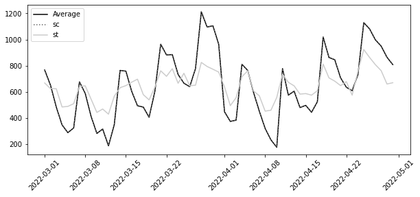

10.2.2 무작위 탐색

from joblib import Parallel, delayed
from toolz import partial

np.random.seed(42)
geo_samples = [np.random.choice(geos, n_tr, replace=False) for _ in range(1000)]

est_combination = partial(get_sc_st_combination, df_sc=df_piv, y_mean_pre=y_avg)

results = Parallel(n_jobs=4)(delayed(est_combination)(geos) for geos in geo_samples)

resulting_geos = min(results, key=lambda x: x.get("loss"))
resulting_geos.get("st_geos")

array(['nova_iguacu', 'belem', 'joinville', 'sao_paulo'], dtype='<U23')

synthetic_tr = SyntheticControl(fit_intercept=True)
synthetic_co = SyntheticControl(fit_intercept=True)

synthetic_tr.fit(df_piv[resulting_geos.get("st_geos")], y_avg)
synthetic_co.fit(df_piv[resulting_geos.get("sc_geos")], y_avg)


plt.figure(figsize=(10, 4))
plt.plot(y_avg, label="Average")
plt.plot(
    y_avg.index,
    synthetic_co.predict(df_piv[resulting_geos.get("sc_geos")]),
    label="sc",
    ls=":",
)
plt.plot(
    y_avg.index, synthetic_tr.predict(df_piv[resulting_geos.get("st_geos")]), label="st"
)


plt.xticks(rotation=45)
plt.legend()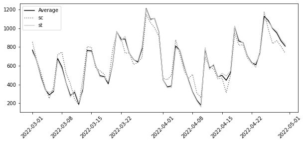

10.3 스위치백 실험

df = pd.read_csv("../data/sb_exp_every.csv")
df.head()

	d	delivery_time	delivery_time_1	delivery_time_0	tau
0	1	2.84	2.84	5.84	-3.0
1	0	4.49	1.49	6.49	-5.0
2	0	7.27	2.27	8.27	-6.0
3	1	5.27	2.27	8.27	-6.0
4	1	5.59	4.59	10.59	-6.0

plt.figure(figsize=(12, 5))
x = df.index
plt.plot(x, df["delivery_time_0"], ls=":", color="0.0", label="Y0")
plt.plot(x, df["delivery_time_1"], ls=":", color="0.8", label="Y1")
plt.plot(x, df["delivery_time"], color="0.4", label="Y")
plt.scatter(
    x[df["d"] == 1],
    df["delivery_time"][df["d"] == 1],
    label="Treated",
    marker="v",
    color="0.4",
)
plt.scatter(
    x[df["d"] == 0],
    df["delivery_time"][df["d"] == 0],
    label="Control",
    marker="o",
    color="0.4",
)
plt.ylabel("delivery_time")
plt.xlabel("Hours")
plt.legend(fontsize=14)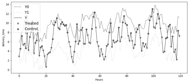

10.3.1 시퀀스의 잠재적 결과

10.3.2 이월 효과의 차수 추정

df_lags = df.assign(**{f"d_l{l}": df["d"].shift(l) for l in range(7)})

df_lags[[f"d_l{l}" for l in range(7)]].head()

	d_l0	d_l1	d_l2	...	d_l4	d_l5	d_l6
0	1	NaN	NaN	...	NaN	NaN	NaN
1	0	1.0	NaN	...	NaN	NaN	NaN
2	0	0.0	1.0	...	NaN	NaN	NaN
3	1	0.0	0.0	...	NaN	NaN	NaN
4	1	1.0	0.0	...	1.0	NaN	NaN

5 rows × 7 columns

model = smf.ols(
    "delivery_time ~" + "+".join([f"d_l{l}" for l in range(7)]), data=df_lags
).fit()

model.summary().tables[1]

	coef	std err	t	P>|t|	[0.025	0.975]
Intercept	9.3270	0.461	20.246	0.000	8.414	10.240
d_l0	-2.9645	0.335	-8.843	0.000	-3.629	-2.300
d_l1	-1.8861	0.339	-5.560	0.000	-2.559	-1.213
d_l2	-1.0013	0.340	-2.943	0.004	-1.676	-0.327
d_l3	0.2594	0.341	0.762	0.448	-0.416	0.935
d_l4	0.1431	0.340	0.421	0.675	-0.531	0.817
d_l5	0.1388	0.340	0.408	0.684	-0.536	0.813
d_l6	0.5588	0.336	1.662	0.099	-0.108	1.225

## remember to remove the intercept
tau_m_hat = model.params[1:].sum()
se_tau_m_hat = np.sqrt((model.bse[1:] ** 2).sum())
print("tau_m:", tau_m_hat)
print("95% CI:", [tau_m_hat - 1.96 * se_tau_m_hat, tau_m_hat + 1.96 * se_tau_m_hat])

tau_m: -4.751686115272022
95% CI: [-6.5087183781545574, -2.9946538523894857]

## selecting lags 0, 1 and 2
tau_m_hat = model.params[1:4].sum()
se_tau_m_hat = np.sqrt((model.bse[1:4] ** 2).sum())
print("tau_m:", tau_m_hat)
print("95% CI:", [tau_m_hat - 1.96 * se_tau_m_hat, tau_m_hat + 1.96 * se_tau_m_hat])

tau_m: -5.8518568954422925
95% CI: [-7.000105171362163, -4.703608619522422]

10.3.3 디자인 기반의 추정

rad_points_3 = np.array([True, False, False] * (2))
rad_points_3

array([ True, False, False,  True, False, False])

rad_points_3.cumsum()

array([1, 1, 1, 2, 2, 2])

from numpy.lib.stride_tricks import sliding_window_view

m = 2
sliding_window_view(rad_points_3.cumsum(), window_shape=m + 1)

array([[1, 1, 1],
       [1, 1, 2],
       [1, 2, 2],
       [2, 2, 2]])

np.diff(sliding_window_view(rad_points_3.cumsum(), 3), axis=1)

array([[0, 0],
       [0, 1],
       [1, 0],
       [0, 0]])

n_rand_windows = np.concatenate(
    [
        [np.nan] * m,
        np.diff(sliding_window_view(rad_points_3.cumsum(), 3), axis=1).sum(axis=1) + 1,
    ]
)

n_rand_windows

array([nan, nan,  1.,  2.,  2.,  1.])

p = 0.5
p**n_rand_windows

array([ nan,  nan, 0.5 , 0.25, 0.25, 0.5 ])

def compute_p(rand_points, m, p=0.5):
    n_windows_last_m = np.concatenate(
        [
            [np.nan] * m,
            np.diff(sliding_window_view(rand_points.cumsum(), m + 1), axis=1).sum(
                axis=1
            )
            + 1,
        ]
    )
    return p**n_windows_last_m


compute_p(np.ones(6) == 1, 2, 0.5)

array([  nan,   nan, 0.125, 0.125, 0.125, 0.125])

rand_points = np.array([True, False, False, True, False, True, False])
compute_p(rand_points, 2, 0.5)

array([ nan,  nan, 0.5 , 0.25, 0.25, 0.25, 0.25])

def last_m_d_equal(d_vec, d, m):
    return np.concatenate(
        [[np.nan] * m, (sliding_window_view(d_vec, m + 1) == d).all(axis=1)]
    )


print(last_m_d_equal([1, 1, 1, 0, 0, 0], 1, m=2))
print(last_m_d_equal([1, 1, 1, 0, 0, 0], 0, m=2))

[nan nan  1.  0.  0.  0.]
[nan nan  0.  0.  0.  1.]

def ipw_switchback(d, y, rand_points, m, p=0.5):
    p_last_m_equal_1 = compute_p(rand_points, m=m, p=p)
    p_last_m_equal_0 = compute_p(rand_points, m=m, p=1 - p)

    last_m_is_1 = last_m_d_equal(d, 1, m)
    last_m_is_0 = last_m_d_equal(d, 0, m)

    y1_rec = y * last_m_is_1 / p_last_m_equal_1
    y0_rec = y * last_m_is_0 / p_last_m_equal_0

    return np.mean((y1_rec - y0_rec)[m:])

ipw_switchback(df["d"], df["delivery_time"], np.ones(len(df)) == 1, m=2, p=0.5)

-7.426440677966101

from matplotlib import pyplot as plt
from statsmodels.tsa.arima_process import ArmaProcess


def gen_d(rand_points, p):
    result = [np.random.binomial(1, p)]

    for t in rand_points[1:]:
        result.append(np.random.binomial(1, p) * t + (1 - t) * result[-1])

    return np.array(result)


def y_given_d(d, effect_params, T, seed=None):
    np.random.seed(seed) if seed is not None else None
    x = np.arange(1, T + 1)
    return (
        np.log(x + 1)
        + 2 * np.sin(x * 2 * np.pi / 24)
        + np.convolve(~d.astype(bool), effect_params)[: -(len(effect_params) - 1)]
        + ArmaProcess([3, 2, 1], 12).generate_sample(T)
    ).round(2)


def gen_data_rand_every():
    effect_params = [3, 2, 1]
    T = 120
    p = 0.5
    m = 2

    d = np.random.binomial(1, 0.5, T)
    y = y_given_d(d, [3, 2, 1], T)
    rand_points = np.ones(T) == 1

    return pd.DataFrame(dict(d=d, y=y, rand_points=rand_points))


def tau_ols(df):
    df_lags = df.assign(**{f"d_l{l}": df["d"].shift(l) for l in range(3)})
    model = smf.ols("y ~" + "+".join([f"d_l{l}" for l in range(3)]), data=df_lags).fit()
    return model.params[1:].sum()


def tau_ipw(df):
    return ipw_switchback(df["d"], df["y"], df["rand_points"], m=2, p=0.5)


np.random.seed(123)
exps_dfs = [gen_data_rand_every() for _ in range(500)]

fig, (ax1, ax2) = plt.subplots(2, 1, sharex=True, figsize=(8, 4))
ols_taus = list(map(tau_ols, exps_dfs))
ax1.hist(ols_taus, label="OLS tau", color="0.5")
ax1.vlines(-6, 0, 120, color="0", label="True tau")
ax1.legend()

ipw_taus = list(map(tau_ipw, exps_dfs))
ax2.hist(ipw_taus, label="IPW tau", color="0.5")
ax2.vlines(-6, 0, 120, color="0")
ax2.legend()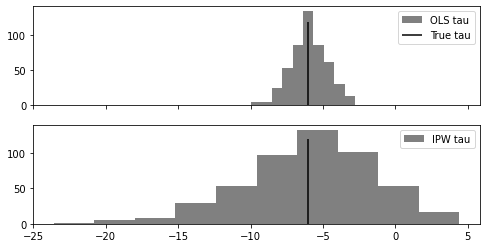

10.3.4 최적의 스위치백 설계

m = 2
T = 12
n = T / m
np.isin(np.arange(1, T + 1), [1] + [i * m + 1 for i in range(2, int(n) - 1)]) * 1

array([1, 0, 0, 0, 1, 0, 1, 0, 1, 0, 0, 0])

m = 3
T = 15
n = T / m
np.isin(np.arange(1, T + 1), [1] + [i * m + 1 for i in range(2, int(n) - 1)]) * 1

array([1, 0, 0, 0, 0, 0, 1, 0, 0, 1, 0, 0, 0, 0, 0])

def gen_d(rand_points, p):
    result = [np.random.binomial(1, p)]

    for t in rand_points[1:]:
        result.append(np.random.binomial(1, p) * t + (1 - t) * result[-1])

    return np.array(result)


T = 120
m = 2


def gen_exp(rand_points, T):
    effect_params = [3, 2, 1]
    p = 0.5

    d = gen_d(rand_points, p=p)
    y = y_given_d(d, [3, 2, 1], T)

    return pd.DataFrame(dict(d=d, y=y, rand_points=rand_points))


every_1 = np.array([True] * T)
every_3 = np.array([True, False, False] * (T // 3))
n = T // m
opt = np.isin(np.arange(1, T + 1), [1] + [i * m + 1 for i in range(2, int(n) - 1)])

np.random.seed(123)
exps_every_1 = [gen_exp(every_1, T) for _ in range(1000)]
exps_every_3 = [gen_exp(every_3, T) for _ in range(1000)]
exps_opt = [gen_exp(opt, T) for _ in range(1000)]

fig, axs = plt.subplots(3, 1, sharex=True, figsize=(12, 6))
ax1, ax2, ax3 = axs.ravel()

taus_every_1_ipw = list(map(tau_ipw, exps_every_1))
ax1.hist(taus_every_1_ipw, label="Every Period", color="0.5")
ax1.set_title(f"Var={np.round(np.var(taus_every_1_ipw), 2)}")
ax1.legend()


taus_every_3_ipw = list(map(tau_ipw, exps_every_3))
ax2.hist(taus_every_3_ipw, label="Every 3 Periods", color="0.5")
ax2.set_title(f"Var={np.round(np.var(taus_every_3_ipw), 2)}")
ax2.legend()

taus_opt_ipw = list(map(tau_ipw, exps_opt))
ax3.hist(taus_opt_ipw, label="Optimal Design", color="0.5")
ax3.set_title(f"Var={np.round(np.var(taus_opt_ipw), 2)}")
ax3.legend()

plt.tight_layout()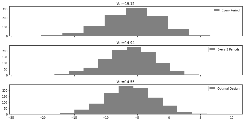

10.3.5 강건한 분산

df_opt = pd.read_csv("../data/sb_exp_opt.csv")
df_opt.head(6)

	rand_points	d	delivery_time
0	True	0	5.84
1	False	0	5.40
2	False	0	8.86
3	False	0	8.79
4	True	0	10.93
5	False	0	7.02

tau_hat = ipw_switchback(
    df_opt["d"], df_opt["delivery_time"], df_opt["rand_points"], m=2, p=0.5
)

tau_hat

-9.921016949152545

np.vstack(np.hsplit(np.array([1, 1, 1, 2, 2, 3]), 3))

array([[1, 1],
       [1, 2],
       [2, 3]])

np.diff(np.vstack(np.hsplit(np.array([1, 1, 0, 0, 0, 0]), 3))[:, 0]) == 0

array([False,  True])

def var_opt_design(d_opt, y_opt, T, m):
    assert (T // m == T / m) & (T // m >= 4), "T must be divisible by m and T/m >= 4"

    # discard 1st block
    y_m_blocks = np.vstack(np.hsplit(y_opt, int(T / m))).sum(axis=1)[1:]

    # take 1st column
    d_m_blocks = np.vstack(np.split(d_opt, int(T / m))[1:])[:, 0]

    return (
        8 * y_m_blocks[0] ** 2
        + (32 * y_m_blocks[1:-1] ** 2 * (np.diff(d_m_blocks) == 0)[:-1]).sum()
        + 8 * y_m_blocks[-1] ** 2
    ) / (T - m) ** 2

se_hat = np.sqrt(var_opt_design(df_opt["d"], df_opt["delivery_time"], T=120, m=2))

[tau_hat - 1.96 * se_hat, tau_hat + 1.96 * se_hat]

[-18.490627362048095, -1.351406536256997]

10.4 요약