7장 - 메타러너

import pandas as pd
import numpy as np
from matplotlib import pyplot as plt
import seaborn as sns
import matplotlib

from fklearn.causal.validation.curves import relative_cumulative_gain_curve
from fklearn.causal.validation.auc import area_under_the_relative_cumulative_gain_curve


from cycler import cycler

color = ["0.0", "0.4", "0.8"]
default_cycler = cycler(color=color)
linestyle = ["-", "--", ":", "-."]
marker = ["o", "v", "d", "p"]

plt.rc("axes", prop_cycle=default_cycler)

7.1 이산형 처치 메타러너

pd.set_option("display.max_columns", 8)

import pandas as pd

data_biased = pd.read_csv("../data/email_obs_data.csv")
data_rnd = pd.read_csv("../data/email_rnd_data.csv")

print(len(data_biased), len(data_rnd))
data_rnd.head()

300000 10000

	mkt_email	next_mnth_pv	age	tenure	...	jewel	books	music_books_movies	health
0	0	244.26	61.0	1.0	...	1	0	0	2
1	0	29.67	36.0	1.0	...	1	0	2	2
2	0	11.73	64.0	0.0	...	0	1	0	1
3	0	41.41	74.0	0.0	...	0	4	1	0
4	0	447.89	59.0	0.0	...	1	1	2	1

5 rows × 27 columns

y = "next_mnth_pv"
T = "mkt_email"
X = list(data_rnd.drop(columns=[y, T]).columns)

train, test = data_biased, data_rnd

7.1.1 T 러너

from lightgbm import LGBMRegressor

np.random.seed(123)

m0 = LGBMRegressor()
m1 = LGBMRegressor()

m0.fit(train.query(f"{T}==0")[X], train.query(f"{T}==0")[y])
m1.fit(train.query(f"{T}==1")[X], train.query(f"{T}==1")[y]);

t_learner_cate_test = test.assign(cate=m1.predict(test[X]) - m0.predict(test[X]))

gain_curve_test = relative_cumulative_gain_curve(
    t_learner_cate_test, T, y, prediction="cate"
)
auc = area_under_the_relative_cumulative_gain_curve(
    t_learner_cate_test, T, y, prediction="cate"
)

plt.figure(figsize=(10, 4))
plt.plot(gain_curve_test, color="C0", label=f"AUC: {auc:.2f}")
plt.hlines(0, 0, 100, linestyle="--", color="black", label="Baseline")

plt.legend()
plt.title("T-Learner")

Text(0.5, 1.0, 'T-Learner')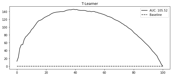

np.random.seed(123)


def g_kernel(x, c=0, s=0.05):
    return np.exp((-((x - c) ** 2)) / s)


n0 = 500
x0 = np.random.uniform(-1, 1, n0)
y0 = np.random.normal(0.3 * g_kernel(x0), 0.1, n0)

n1 = 50
x1 = np.random.uniform(-1, 1, n1)
y1 = np.random.normal(0.3 * g_kernel(x1), 0.1, n1) + 1

df = pd.concat(
    [pd.DataFrame(dict(x=x0, y=y0, t=0)), pd.DataFrame(dict(x=x1, y=y1, t=1))]
).sort_values(by="x")

m0 = LGBMRegressor(min_child_samples=25)
m1 = LGBMRegressor(min_child_samples=25)

m0.fit(x0.reshape(-1, 1), y0)
m1.fit(x1.reshape(-1, 1), y1)

m0_hat = m0.predict(df.query("t==0")[["x"]])
m1_hat = m1.predict(df.query("t==1")[["x"]])

fig, (ax1, ax2) = plt.subplots(2, 1, figsize=(10, 10))

ax1.scatter(x0, y0, alpha=0.5, label="T=0", marker=marker[0], color=color[1])
ax1.scatter(x1, y1, alpha=0.7, label="T=1", marker=marker[1], color=color[0])

ax1.plot(
    df.query("t==0")[["x"]],
    m0_hat,
    color="black",
    linestyle="solid",
    label="$\hat{\mu}_0$",
)
ax1.plot(
    df.query("t==1")[["x"]],
    m1_hat,
    color="black",
    linestyle="--",
    label="$\hat{\mu}_1$",
)

ax1.set_ylabel("Y")
ax1.set_xlabel("X")
ax1.legend(fontsize=14)
tau_0 = m1.predict(df.query("t==0")[["x"]]) - df.query("t==0")["y"]
tau_1 = df.query("t==1")["y"] - m0.predict(df.query("t==1")[["x"]])

ax2.scatter(
    df.query("t==0")[["x"]],
    tau_0,
    label="$\hat{\\tau_0}$",
    alpha=0.5,
    marker=marker[0],
    color=color[1],
)
ax2.scatter(
    df.query("t==1")[["x"]],
    tau_1,
    label="$\hat{\\tau_1}$",
    alpha=0.7,
    marker=marker[1],
    color=color[0],
)

ax2.plot(
    df[["x"]],
    m1.predict(df[["x"]]) - m0.predict(df[["x"]]),
    label="$\hat{CATE}$",
    color="black",
)

ax2.set_ylabel("Estimated Effect")
ax2.set_xlabel("X")
ax2.legend(fontsize=14)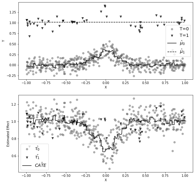

7.1.2 X 러너

from sklearn.linear_model import LogisticRegression

np.random.seed(42)

mu_tau0 = LGBMRegressor(min_child_samples=25)
mu_tau1 = LGBMRegressor(min_child_samples=25)

mu_tau0.fit(df.query("t==0")[["x"]], tau_0)
mu_tau1.fit(df.query("t==1")[["x"]], tau_1)

mu_tau0_hat = mu_tau0.predict(df.query("t==0")[["x"]])
mu_tau1_hat = mu_tau1.predict(df.query("t==1")[["x"]])

plt.figure(figsize=(10, 4))
plt.scatter(
    df.query("t==0")[["x"]],
    tau_0,
    label="$\hat{\\tau_0}$",
    alpha=0.5,
    marker=marker[0],
    color=color[1],
)
plt.scatter(
    df.query("t==1")[["x"]],
    tau_1,
    label="$\hat{\\tau_1}$",
    alpha=0.8,
    marker=marker[1],
    color=color[0],
)
plt.plot(
    df.query("t==0")[["x"]],
    mu_tau0_hat,
    color="black",
    linestyle="solid",
    label="$\hat{\mu}\\tau 0$",
)
plt.plot(
    df.query("t==1")[["x"]],
    mu_tau1_hat,
    color="black",
    linestyle="dashed",
    label="$\hat{\mu}\\tau_1$",
)
plt.ylabel("Estimated Effect")
plt.xlabel("X")
plt.legend(fontsize=14)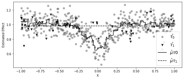

plt.figure(figsize=(10, 4))

ps_model = LogisticRegression(penalty="none")
ps_model.fit(df[["x"]], df["t"])

ps = ps_model.predict_proba(df[["x"]])[:, 1]

cate = (1 - ps) * mu_tau1.predict(df[["x"]]) + ps * mu_tau0.predict(df[["x"]])

plt.scatter(
    df.query("t==0")[["x"]],
    tau_0,
    label="$\hat{\\tau_0}$",
    alpha=0.5,
    s=100 * (ps[df["t"] == 0]),
    marker=marker[0],
    color=color[1],
)
plt.scatter(
    df.query("t==1")[["x"]],
    tau_1,
    label="$\hat{\\tau_1}$",
    alpha=0.5,
    s=100 * (1 - ps[df["t"] == 1]),
    marker=marker[1],
    color=color[0],
)

plt.plot(df[["x"]], cate, label="x-learner", color="black")
plt.ylabel("Estimated Effect")
plt.xlabel("X")
plt.legend(fontsize=14)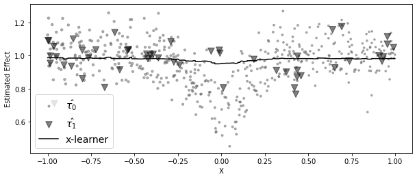

from sklearn.linear_model import LogisticRegression
from lightgbm import LGBMRegressor

# propensity score model
ps_model = LogisticRegression(penalty="none")
ps_model.fit(train[X], train[T])


# first stage models
train_t0 = train.query(f"{T}==0")
train_t1 = train.query(f"{T}==1")

m0 = LGBMRegressor()
m1 = LGBMRegressor()

np.random.seed(123)

m0.fit(
    train_t0[X],
    train_t0[y],
    sample_weight=1 / ps_model.predict_proba(train_t0[X])[:, 0],
)

m1.fit(
    train_t1[X],
    train_t1[y],
    sample_weight=1 / ps_model.predict_proba(train_t1[X])[:, 1],
);

# second stage
tau_hat_0 = m1.predict(train_t0[X]) - train_t0[y]
tau_hat_1 = train_t1[y] - m0.predict(train_t1[X])

m_tau_0 = LGBMRegressor()
m_tau_1 = LGBMRegressor()

np.random.seed(123)

m_tau_0.fit(train_t0[X], tau_hat_0)
m_tau_1.fit(train_t1[X], tau_hat_1);

# estimate the CATE
ps_test = ps_model.predict_proba(test[X])[:, 1]

x_cate_test = test.assign(
    cate=(ps_test * m_tau_0.predict(test[X]) + (1 - ps_test) * m_tau_1.predict(test[X]))
)

gain_curve_test = relative_cumulative_gain_curve(x_cate_test, T, y, prediction="cate")
auc = area_under_the_relative_cumulative_gain_curve(
    x_cate_test, T, y, prediction="cate"
)

plt.figure(figsize=(10, 4))
plt.plot(gain_curve_test, color="C0", label=f"AUC: {auc:.2f}")
plt.hlines(0, 0, 100, linestyle="--", color="black", label="Baseline")

plt.legend()
plt.title("X-Learner")

Text(0.5, 1.0, 'X-Learner')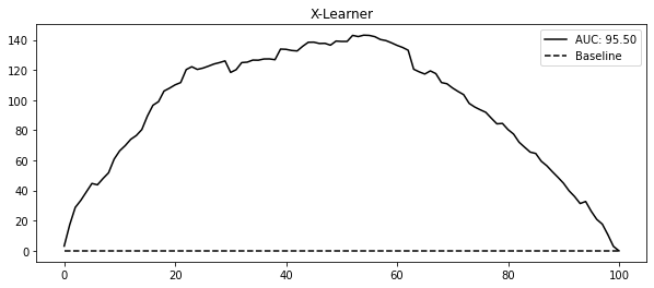

7.2 연속형 처치 메타러너

data_cont = pd.read_csv("../data/discount_data.csv")
data_cont.head()

	rest_id	day	month	weekday	...	is_nov	competitors_price	discounts	sales
0	0	2016-01-01	1	4	...	False	2.88	0	79.0
1	0	2016-01-02	1	5	...	False	2.64	0	57.0
2	0	2016-01-03	1	6	...	False	2.08	5	294.0
3	0	2016-01-04	1	0	...	False	3.37	15	676.5
4	0	2016-01-05	1	1	...	False	3.79	0	66.0

5 rows × 11 columns

train = data_cont.query("day<'2018-01-01'")
test = data_cont.query("day>='2018-01-01'")

7.2.1 S 러너

X = ["month", "weekday", "is_holiday", "competitors_price"]
T = "discounts"
y = "sales"

np.random.seed(123)
s_learner = LGBMRegressor()
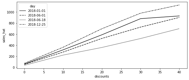
s_learner.fit(train[X + [T]], train[y]);

t_grid = pd.DataFrame(dict(key=1, discounts=np.array([0, 10, 20, 30, 40])))

test_cf = (
    test.drop(columns=["discounts"])
    .assign(key=1)
    .merge(t_grid)
    # make predictions after expansion
    .assign(sales_hat=lambda d: s_learner.predict(d[X + [T]]))
)

test_cf.head(8)

	rest_id	day	month	weekday	...	sales	key	discounts	sales_hat
0	0	2018-01-01	1	0	...	251.5	1	0	67.957972
1	0	2018-01-01	1	0	...	251.5	1	10	444.245941
2	0	2018-01-01	1	0	...	251.5	1	20	793.045769
3	0	2018-01-01	1	0	...	251.5	1	30	1279.640793
4	0	2018-01-01	1	0	...	251.5	1	40	1512.630767
5	0	2018-01-02	1	1	...	541.0	1	0	65.672080
6	0	2018-01-02	1	1	...	541.0	1	10	495.669220
7	0	2018-01-02	1	1	...	541.0	1	20	1015.401471

8 rows × 13 columns

days = ["2018-12-25", "2018-01-01", "2018-06-01", "2018-06-18"]

plt.figure(figsize=(10, 4))
sns.lineplot(
    data=test_cf.query("day.isin(@days)").query("rest_id==2"),
    palette="gray",
    y="sales_hat",
    x="discounts",
    style="day",
);

from toolz import curry


@curry
def linear_effect(df, y, t):
    return np.cov(df[y], df[t])[0, 1] / df[t].var()


cate = (
    test_cf.groupby(["rest_id", "day"])
    .apply(linear_effect(t="discounts", y="sales_hat"))
    .rename("cate")
)

test_s_learner_pred = test.set_index(["rest_id", "day"]).join(cate)

test_s_learner_pred.head()

		month	weekday	weekend	is_holiday	...	competitors_price	discounts	sales	cate
rest_id	day
0	2018-01-01	1	0	False	True	...	4.92	5	251.5	37.247404
	2018-01-02	1	1	False	False	...	3.06	10	541.0	40.269854
	2018-01-03	1	2	False	False	...	4.61	10	431.0	37.412988
	2018-01-04	1	3	False	False	...	4.84	20	760.0	38.436815
	2018-01-05	1	4	False	False	...	6.29	0	78.0	31.428603

5 rows × 10 columns

from fklearn.causal.validation.auc import area_under_the_relative_cumulative_gain_curve
from fklearn.causal.validation.curves import relative_cumulative_gain_curve

gain_curve_test = relative_cumulative_gain_curve(
    test_s_learner_pred, T, y, prediction="cate"
)
auc = area_under_the_relative_cumulative_gain_curve(
    test_s_learner_pred, T, y, prediction="cate"
)

plt.figure(figsize=(10, 4))
plt.plot(gain_curve_test, color="C0", label=f"AUC: {auc:.2f}")
plt.hlines(0, 0, 100, linestyle="--", color="black", label="Baseline")

plt.legend()
plt.title("S-Learner")

Text(0.5, 1.0, 'S-Learner')

np.random.seed(123)


def sim_s_learner_ate():
    n = 10000
    nx = 20

    X = np.random.normal(0, 1, (n, nx))
    coefs_y = np.random.uniform(-1, 1, nx)
    coefs_t = np.random.uniform(-0.5, 0.5, nx)

    ps = 1 / (1 + np.exp(-(X.dot(coefs_t))))
    t = np.random.binomial(1, ps)
    te = 1

    y = np.random.normal(t * te + X.dot(coefs_y), 1)

    s_learner = LGBMRegressor(max_depth=5, n_jobs=4)
    s_learner.fit(np.concatenate([X, t.reshape(-1, 1)], axis=1), y)
    ate_hat = (
        s_learner.predict(np.concatenate([X, np.ones((n, 1))], axis=1))
        - s_learner.predict(np.concatenate([X, np.zeros((n, 1))], axis=1))
    ).mean()

    return ate_hat


ates = [sim_s_learner_ate() for _ in range(500)]

plt.figure(figsize=(10, 4))
plt.hist(ates, alpha=0.5, bins=20, label="Simulations")
plt.vlines(1, 0, 70, label="True ATE")
plt.legend()
plt.xlabel("ATE")
plt.title("500 Simulations")

Text(0.5, 1.0, '500 Simulations')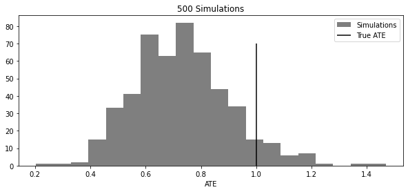

7.2.2 이중/편향 제거 머신러닝

from sklearn.model_selection import cross_val_predict

X = ["month", "weekday", "is_holiday", "competitors_price"]
T = "discounts"
y = "sales"

debias_m = LGBMRegressor()
denoise_m = LGBMRegressor()

t_res = train[T] - cross_val_predict(debias_m, train[X], train[T], cv=5)
y_res = train[y] - cross_val_predict(denoise_m, train[X], train[y], cv=5)

import statsmodels.api as sm

sm.OLS(y_res, t_res).fit().summary().tables[1]

	coef	std err	t	P>|t|	[0.025	0.975]
discounts	31.4615	0.151	208.990	0.000	31.166	31.757

이중 머신러닝으로 CATE 추정

y_star = y_res / t_res
w = t_res**2

cate_model = LGBMRegressor().fit(train[X], y_star, sample_weight=w)

test_r_learner_pred = test.assign(cate=cate_model.predict(test[X]))

gain_curve_test = relative_cumulative_gain_curve(
    test_r_learner_pred, T, y, prediction="cate"
)
auc = area_under_the_relative_cumulative_gain_curve(
    test_r_learner_pred, T, y, prediction="cate"
)

plt.figure(figsize=(10, 4))
plt.plot(gain_curve_test, color="C0", label=f"AUC: {auc:.2f}")
plt.hlines(0, 0, 100, linestyle="--", color="black", label="Baseline")

plt.legend()
plt.title("R-Learner")

Text(0.5, 1.0, 'R-Learner')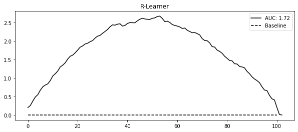

이중 머신러닝에 대한 시각적인 직관

np.random.seed(123)
n = 5000

x_h = np.random.randint(1, 4, n)
x_c = np.random.uniform(-1, 1, n)

t = np.random.normal(10 + 1 * x_c + 3 * x_c**2 + x_c**3, 0.3)
y = np.random.normal(t + x_h * t - 5 * x_c - x_c**2 - x_c**3, 0.3)

df_sim = pd.DataFrame(dict(x_h=x_h, x_c=x_c, t=t, y=y))

plt.figure(figsize=(10, 5))
cmap = matplotlib.colors.LinearSegmentedColormap.from_list("", ["0.1", "0.5", "0.9"])

sns.scatterplot(data=df_sim, y="y", x="t", hue="x_c", style="x_h", palette=cmap)
plt.legend(fontsize=14)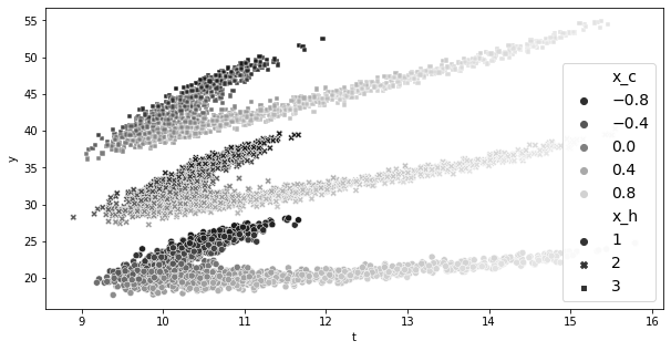

debias_m = LGBMRegressor(max_depth=3)
denoise_m = LGBMRegressor(max_depth=3)

t_res = cross_val_predict(debias_m, df_sim[["x_c"]], df_sim["t"], cv=10)

y_res = cross_val_predict(denoise_m, df_sim[["x_c", "x_h"]], df_sim["y"], cv=10)

df_res = df_sim.assign(t_res=df_sim["t"] - t_res, y_res=df_sim["y"] - y_res)

import statsmodels.formula.api as smf

smf.ols("y_res~t_res", data=df_res).fit().params["t_res"]

3.045230146006292

fig, (ax1, ax2) = plt.subplots(1, 2, figsize=(15, 5))

ax1 = sns.scatterplot(
    data=df_res,
    y="y_res",
    x="t_res",
    hue="x_c",
    style="x_h",
    alpha=0.5,
    ax=ax1,
    palette=cmap,
)

h, l = ax1.get_legend_handles_labels()
ax1.legend(fontsize=14)

sns.scatterplot(
    data=df_res, y="y_res", x="t_res", hue="x_h", ax=ax2, alpha=0.5, palette=cmap
)
ax2.legend(fontsize=14)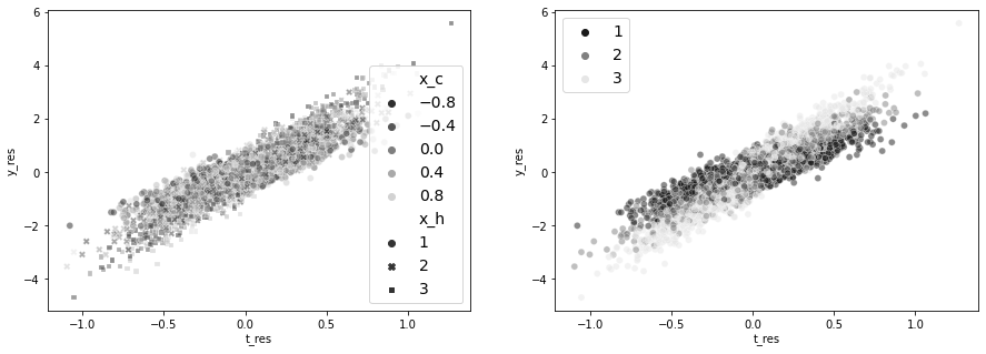

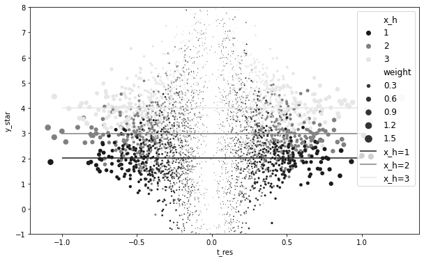
df_star = df_res.assign(
    y_star=df_res["y_res"] / df_res["t_res"],
    weight=df_res["t_res"] ** 2,
)

for x in range(1, 4):
    cate = np.average(
        df_star.query(f"x_h=={x}")["y_star"],
        weights=df_star.query(f"x_h=={x}")["weight"],
    )

    print(f"CATE x_h={x}", cate)

CATE x_h=1 2.019759619990067
CATE x_h=2 2.974967932350952
CATE x_h=3 3.9962382855476957

plt.figure(figsize=(10, 6))

(
    sns.scatterplot(
        data=df_star,
        palette=cmap,
        y="y_star",
        x="t_res",
        hue="x_h",
        size="weight",
        sizes=(1, 100),
    ),
)

plt.hlines(
    np.average(
        df_star.query("x_h==1")["y_star"], weights=df_star.query("x_h==1")["weight"]
    ),
    -1,
    1,
    label="x_h=1",
    color="0.1",
)

plt.hlines(
    np.average(
        df_star.query("x_h==2")["y_star"], weights=df_star.query("x_h==2")["weight"]
    ),
    -1,
    1,
    label="x_h=2",
    color="0.5",
)

plt.hlines(
    np.average(
        df_star.query("x_h==3")["y_star"], weights=df_star.query("x_h==3")["weight"]
    ),
    -1,
    1,
    label="x_h=3",
    color="0.9",
)

plt.ylim(-1, 8)

plt.legend(fontsize=12)

7.3 요약