8장 - 이중차분법

8.1 패널데이터

from toolz import *

import pandas as pd
import numpy as np

import statsmodels.formula.api as smf

import seaborn as sns
from matplotlib import pyplot as plt

from cycler import cycler

color = ["0.0", "0.4", "0.8"]
default_cycler = cycler(color=color)
linestyle = ["-", "--", ":", "-."]
marker = ["o", "v", "d", "p"]

plt.rc("axes", prop_cycle=default_cycler)

mkt_data = pd.read_csv("../data/short_offline_mkt_south.csv").astype(
    {"date": "datetime64[ns]"}
)

mkt_data.head()

	date	city	region	treated	tau	downloads	post
0	2021-05-01	5	S	0	0.0	51.0	0
1	2021-05-02	5	S	0	0.0	51.0	0
2	2021-05-03	5	S	0	0.0	51.0	0
3	2021-05-04	5	S	0	0.0	50.0	0
4	2021-05-05	5	S	0	0.0	49.0	0

(
    mkt_data.assign(w=lambda d: d["treated"] * d["post"])
    .groupby(["w"])
    .agg({"date": [min, max]})
)

	date
	min	max
w
0	2021-05-01	2021-06-01
1	2021-05-15	2021-06-01

8.2 표준 이중차분법

이중차분법(DiD)은 처치군의 전후 변화에서 대조군의 전후 변화를 차감하여 순수한 처치 효과를 계산합니다.

did_data = mkt_data.groupby(["treated", "post"]).agg(
    {"downloads": "mean", "date": "min"}
)

did_data

		downloads	date
treated	post
0	0	50.335034	2021-05-01
	1	50.556878	2021-05-15
1	0	50.944444	2021-05-01
	1	51.858025	2021-05-15

y0_est = (
    did_data.loc[1].loc[0, "downloads"]  # treated baseline
    # control evolution
    + did_data.loc[0].diff().loc[1, "downloads"]
)

att = did_data.loc[1].loc[1, "downloads"] - y0_est
att

0.6917359536407233

mkt_data.query("post==1").query("treated==1")["tau"].mean()

0.7660316402518457

8.2.1 이중차분법과 결과 변화

처치 전후의 결과값 변화량이 처치 여부에 따라 어떻게 다른지 비교하는 것이 이중차분법의 핵심 원리입니다.

pre = mkt_data.query("post==0").groupby("city")["downloads"].mean()
post = mkt_data.query("post==1").groupby("city")["downloads"].mean()

delta_y = (
    (post - pre)
    .rename("delta_y")
    .to_frame()
    # add the treatment dummy
    .join(mkt_data.groupby("city")["treated"].max())
)

delta_y.tail()

	delta_y	treated
city
192	0.555556	0
193	0.166667	0
195	0.420635	0
196	0.119048	0
197	1.595238	1

(
    delta_y.query("treated==1")["delta_y"].mean()
    - delta_y.query("treated==0")["delta_y"].mean()
)

0.6917359536407155

did_plt = did_data.reset_index()


plt.figure(figsize=(10, 4))

sns.scatterplot(
    data=did_plt.query("treated==0"),
    x="date",
    y="downloads",
    s=100,
    color="C0",
    marker="s",
)
sns.lineplot(
    data=did_plt.query("treated==0"),
    x="date",
    y="downloads",
    label="Control",
    color="C0",
)

sns.scatterplot(
    data=did_plt.query("treated==1"),
    x="date",
    y="downloads",
    s=100,
    color="C1",
    marker="x",
)
sns.lineplot(
    data=did_plt.query("treated==1"),
    x="date",
    y="downloads",
    label="Treated",
    color="C1",
)

plt.plot(
    did_data.loc[1, "date"],
    [did_data.loc[1, "downloads"][0], y0_est],
    color="C2",
    linestyle="dashed",
    label="Y(0)|D=1",
)
plt.scatter(
    did_data.loc[1, "date"], [did_data.loc[1, "downloads"][0], y0_est], color="C2", s=50
)

plt.xticks(rotation=45)
plt.legend()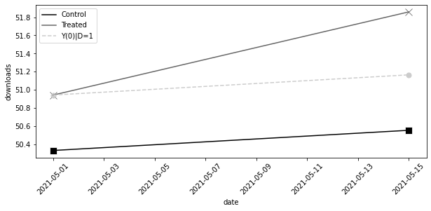

8.2.2 이중차분법과 OLS

did_data = (
    mkt_data.groupby(["city", "post"])
    .agg({"downloads": "mean", "date": "min", "treated": "max"})
    .reset_index()
)

did_data.head()

	city	post	downloads	date	treated
0	5	0	50.642857	2021-05-01	0
1	5	1	50.166667	2021-05-15	0
2	15	0	49.142857	2021-05-01	0
3	15	1	49.166667	2021-05-15	0
4	20	0	48.785714	2021-05-01	0

smf.ols("downloads ~ treated*post", data=did_data).fit().params["treated:post"]

0.6917359536406904

8.2.3 이중차분법과 고정효과

m = smf.ols("downloads ~ treated:post + C(city) + C(post)", data=did_data).fit()

m.params["treated:post"]

0.6917359536407091

8.2.4 이중차분법과 블록 디자인

import matplotlib.ticker as plticker


fig, (ax1, ax2) = plt.subplots(2, 1, figsize=(9, 12), sharex=True)

heat_plt = (
    mkt_data.assign(treated=lambda d: d.groupby("city")["treated"].transform(max))
    .astype({"date": "str"})
    .assign(treated=mkt_data["treated"] * mkt_data["post"])
    .pivot("city", "date", "treated")
    .reset_index()
    .sort_values(max(mkt_data["date"].astype(str)), ascending=False)
    .reset_index()
    .drop(columns=["city"])
    .rename(columns={"index": "city"})
    .set_index("city")
)


sns.heatmap(heat_plt, cmap="gray", linewidths=0.01, linecolor="0.5", ax=ax1, cbar=False)

ax1.set_title("Treatment Assignment")


sns.lineplot(
    data=mkt_data.astype({"date": "str"}),
    x="date",
    y="downloads",
    hue="treated",
    ax=ax2,
)

loc = plticker.MultipleLocator(base=2.0)
# ax2.xaxis.set_major_locator(loc)
ax2.vlines(
    "2021-05-15",
    mkt_data["downloads"].min(),
    mkt_data["downloads"].max(),
    color="black",
    ls="dashed",
    label="Interv.",
)
ax2.set_title("Outcome Over Time")

plt.xticks(rotation=50);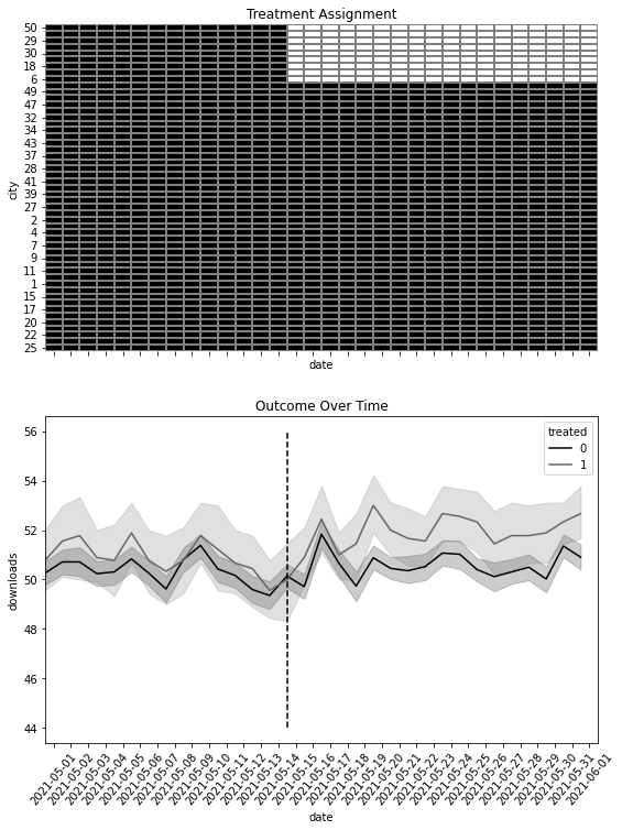

m = smf.ols("downloads ~ treated*post", data=mkt_data).fit()

m.params["treated:post"]

0.6917359536407226

m = smf.ols("downloads ~ treated:post + C(city) + C(date)", data=mkt_data).fit()

m.params["treated:post"]

0.6917359536407017

8.2.5 추론

m = smf.ols("downloads ~ treated:post + C(city) + C(date)", data=mkt_data).fit(
    cov_type="cluster", cov_kwds={"groups": mkt_data["city"]}
)

print("ATT:", m.params["treated:post"])
m.conf_int().loc["treated:post"]

ATT: 0.6917359536407017

0    0.296101
1    1.087370
Name: treated:post, dtype: float64

m = smf.ols("downloads ~ treated:post + C(city) + C(date)", data=mkt_data).fit()

print("ATT:", m.params["treated:post"])
m.conf_int().loc["treated:post"]

ATT: 0.6917359536407017

0    0.478014
1    0.905457
Name: treated:post, dtype: float64

m = smf.ols("downloads ~ treated:post + C(city) + C(date)", data=did_data).fit(
    cov_type="cluster", cov_kwds={"groups": did_data["city"]}
)

print("ATT:", m.params["treated:post"])
m.conf_int().loc["treated:post"]

ATT: 0.6917359536407091

0    0.138188
1    1.245284
Name: treated:post, dtype: float64

def block_sample(df, unit_col):
    units = df[unit_col].unique()
    sample = np.random.choice(units, size=len(units), replace=True)

    return df.set_index(unit_col).loc[sample].reset_index(level=[unit_col])

from joblib import Parallel, delayed


def block_bootstrap(data, est_fn, unit_col, rounds=200, seed=123, pcts=[2.5, 97.5]):
    np.random.seed(seed)

    stats = Parallel(n_jobs=4)(
        delayed(est_fn)(block_sample(data, unit_col=unit_col)) for _ in range(rounds)
    )

    return np.percentile(stats, pcts)

def est_fn(df):
    m = smf.ols("downloads ~ treated:post + C(city) + C(date)", data=df).fit()
    return m.params["treated:post"]


block_bootstrap(mkt_data, est_fn, "city")

array([0.23162214, 1.14002646])

8.3 식별 가정

8.3.1 평행 추세

fig, (ax1, ax2, ax3) = plt.subplots(1, 3, figsize=(20, 7))

obs_df = pd.DataFrame(
    dict(
        period=[2, 3, 2, 3],
        treated=[0, 0, 1, 1],
        y=[4, 6, 10, 16],
    )
)

baseline = 10 - 4


plt_d1 = pd.DataFrame(
    dict(
        period=[1, 2, 3, 4, 1, 2, 3, 4],
        treated=[0, 0, 0, 0, 1, 1, 1, 1],
        y=[2, 4, 6, 8, 8, 10, 12, 14],
    )
)

sns.lineplot(
    data=plt_d1,
    x="period",
    y="y",
    hue="treated",
    linestyle="dashed",
    legend=None,
    ax=ax1,
)
sns.lineplot(data=obs_df, x="period", y="y", hue="treated", legend=None, ax=ax1)
sns.lineplot(
    data=obs_df.assign(y=obs_df["y"] + baseline).query("treated==0"),
    x="period",
    y="y",
    legend=None,
    ax=ax1,
    color="C0",
    linestyle="dotted",
)

sns.scatterplot(
    data=obs_df, x="period", y="y", hue="treated", style="treated", s=100, ax=ax1
)
ax1.set_title("Parallel Trends")


plt_d2 = pd.DataFrame(
    dict(
        period=[1, 2, 3, 4, 1, 2, 3, 4],
        treated=[0, 0, 0, 0, 1, 1, 1, 1],
        y=[2, 4, 6, 8, 9, 10, 11, 12],
    )
)

sns.lineplot(
    data=plt_d2,
    x="period",
    y="y",
    hue="treated",
    linestyle="dashed",
    legend=None,
    ax=ax2,
)
sns.lineplot(data=obs_df, x="period", y="y", hue="treated", legend=None, ax=ax2)
sns.scatterplot(
    data=obs_df, x="period", y="y", hue="treated", style="treated", s=100, ax=ax2
)
sns.lineplot(
    data=obs_df.assign(y=obs_df["y"] + baseline).query("treated==0"),
    x="period",
    y="y",
    legend=None,
    ax=ax2,
    color="C0",
    linestyle="dotted",
)

ax2.set_title("Diverging Trends")


non_lin = np.log
non_lin_obs = obs_df.assign(y=non_lin(obs_df["y"]))

plt_d3 = pd.DataFrame(
    dict(
        period=[1, 2, 3, 4, 1, 2, 3, 4],
        treated=[0, 0, 0, 0, 1, 1, 1, 1],
        y=non_lin([2, 4, 6, 8, 8, 10, 12, 14]),
    )
)


sns.lineplot(
    data=plt_d3,
    x="period",
    y="y",
    hue="treated",
    linestyle="dashed",
    legend=None,
    ax=ax3,
)
sns.lineplot(data=non_lin_obs, x="period", y="y", hue="treated", legend=None, ax=ax3)
sns.scatterplot(
    data=non_lin_obs, x="period", y="y", hue="treated", style="treated", s=100, ax=ax3
)
sns.lineplot(
    x=[2, 3],
    y=non_lin_obs.query("treated==1 & period==2")["y"].values
    - non_lin_obs.query("treated==0 & period==2")["y"].values
    + non_lin_obs.query("treated==0")["y"],
    color="C0",
    linestyle="dotted",
)


ax3.set_title("Log Scale")
ax3.set_ylabel("Log(y)")

Text(0, 0.5, 'Log(y)')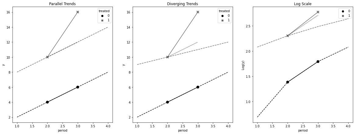

8.3.2 비기대 가정과 SUTVA

8.3.3 강외생성

8.3.4 시간에 따라 변하지 않는 교란 요인

8.3.5 피드백 없음

8.3.6 이월 효과와 시차종속변수 없음

8.4 시간에 따른 효과 변동

def did_date(df, date):
    df_date = (
        df.query("date==@date | post==0")
        .query("date <= @date")
        .assign(post=lambda d: (d["date"] == date).astype(int))
    )

    m = smf.ols("downloads ~ I(treated*post) + C(city) + C(date)", data=df_date).fit(
        cov_type="cluster", cov_kwds={"groups": df_date["city"]}
    )

    att = m.params["I(treated * post)"]
    ci = m.conf_int().loc["I(treated * post)"]

    return pd.DataFrame({"att": att, "ci_low": ci[0], "ci_up": ci[1]}, index=[date])

post_dates = sorted(mkt_data["date"].unique())[1:]

atts = pd.concat([did_date(mkt_data, date) for date in post_dates])

atts.head()

	att	ci_low	ci_up
2021-05-02	0.325397	-0.491741	1.142534
2021-05-03	0.384921	-0.388389	1.158231
2021-05-04	-0.156085	-1.247491	0.935321
2021-05-05	-0.299603	-0.949935	0.350729
2021-05-06	0.347619	0.013115	0.682123

plt.figure(figsize=(10, 4))
plt.plot(atts.index, atts["att"], label="Est. ATTs")

plt.fill_between(atts.index, atts["ci_low"], atts["ci_up"], alpha=0.1)

plt.vlines(
    pd.to_datetime("2021-05-15"), -2, 3, linestyle="dashed", label="intervention"
)
plt.hlines(0, atts.index.min(), atts.index.max(), linestyle="dotted")

plt.plot(
    atts.index,
    mkt_data.query("treated==1").groupby("date")[["tau"]].mean().values[1:],
    color="0.6",
    ls="-.",
    label="$\\tau$",
)

plt.xticks(rotation=45)
plt.title("DID ATTs Over Time")
plt.legend()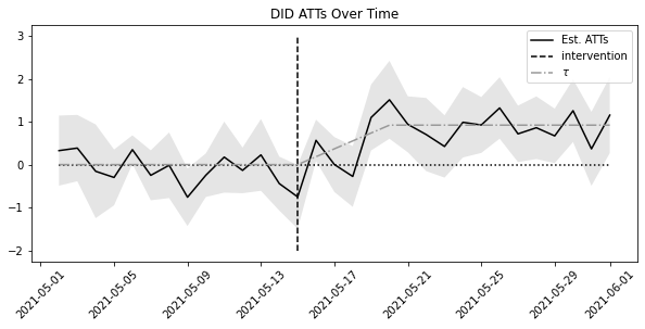

8.5 이중차분법과 공변량

mkt_data_all = pd.read_csv("../data/short_offline_mkt_all_regions.csv").astype(
    {"date": "datetime64[ns]"}
)

plt.figure(figsize=(15, 6))
sns.lineplot(
    data=mkt_data_all.groupby(["date", "region", "treated"])[["downloads"]]
    .mean()
    .reset_index(),
    x="date",
    y="downloads",
    hue="region",
    style="treated",
    palette="gray",
)

plt.vlines(pd.to_datetime("2021-05-15"), 15, 55, ls="dotted", label="Intervention")
plt.legend(fontsize=14)

plt.xticks(rotation=25);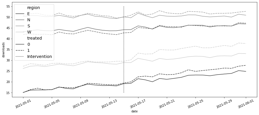

print("True ATT: ", mkt_data_all.query("treated*post==1")["tau"].mean())

m = smf.ols("downloads ~ treated:post + C(city) + C(date)", data=mkt_data_all).fit()

print("Estimated ATT:", m.params["treated:post"])

True ATT:  1.7208921056102682
Estimated ATT: 2.068391984256296

m = smf.ols(
    "downloads ~ treated:post + C(city) + C(date) + C(region)", data=mkt_data_all
).fit()
m.params["treated:post"]

2.071153674125536

m_saturated = smf.ols("downloads ~ (post*treated)*C(region)", data=mkt_data_all).fit()

atts = m_saturated.params[m_saturated.params.index.str.contains("post:treated")]
atts

post:treated                   1.676808
post:treated:C(region)[T.N]   -0.343667
post:treated:C(region)[T.S]   -0.985072
post:treated:C(region)[T.W]    1.369363
dtype: float64

reg_size = mkt_data_all.groupby("region").size() / len(mkt_data_all["date"].unique())

base = atts[0]

np.array(
    [reg_size[0] * base]
    + [(att + base) * size for att, size in zip(atts[1:], reg_size[1:])]
).sum() / sum(reg_size)

1.6940400451471818

m = smf.ols("downloads ~ post*(treated + C(region))", data=mkt_data_all).fit()

m.summary().tables[1]

	coef	std err	t	P>|t|	[0.025	0.975]
Intercept	17.3522	0.101	172.218	0.000	17.155	17.550
C(region)[T.N]	26.2770	0.137	191.739	0.000	26.008	26.546
C(region)[T.S]	33.0815	0.135	245.772	0.000	32.818	33.345
C(region)[T.W]	10.7118	0.135	79.581	0.000	10.448	10.976
post	4.9807	0.134	37.074	0.000	4.717	5.244
post:C(region)[T.N]	-3.3458	0.183	-18.310	0.000	-3.704	-2.988
post:C(region)[T.S]	-4.9334	0.179	-27.489	0.000	-5.285	-4.582
post:C(region)[T.W]	-1.5408	0.179	-8.585	0.000	-1.893	-1.189
treated	0.0503	0.117	0.429	0.668	-0.179	0.280
post:treated	1.6811	0.156	10.758	0.000	1.375	1.987

8.6 이중 강건 이중차분법

8.6.1 성향점수 모델

import warnings

warnings.filterwarnings("ignore")

unit_df = (
    mkt_data_all
    # keep only the first date
    .astype({"date": str})
    .query(f"date=='{mkt_data_all['date'].astype(str).min()}'")
    .drop(columns=["date"])
)  # just to avoid confusion

ps_model = smf.logit("treated~C(region)", data=unit_df).fit(disp=0)

8.6.2 델타 결과 모델

delta_y = (
    mkt_data_all.query("post==1").groupby("city")["downloads"].mean()
    - mkt_data_all.query("post==0").groupby("city")["downloads"].mean()
)

df_delta_y = unit_df.set_index("city").join(delta_y.rename("delta_y"))

outcome_model = smf.ols("delta_y ~ C(region)", data=df_delta_y).fit()

8.6.3 최종 결과

df_dr = df_delta_y.assign(y_hat=lambda d: outcome_model.predict(d)).assign(
    ps=lambda d: ps_model.predict(d)
)

df_dr.head()

	region	treated	tau	downloads	post	delta_y	y_hat	ps
city
1	W	0	0.0	27.0	0	3.087302	3.736539	0.176471
2	N	0	0.0	40.0	0	1.436508	1.992570	0.212766
3	W	0	0.0	30.0	0	2.761905	3.736539	0.176471
4	W	0	0.0	26.0	0	3.396825	3.736539	0.176471
5	S	0	0.0	51.0	0	-0.476190	0.343915	0.176471

tr = df_dr.query("treated==1")
co = df_dr.query("treated==0")

dy1_treat = (tr["delta_y"] - tr["y_hat"]).mean()

w_cont = co["ps"] / (1 - co["ps"])
dy0_treat = np.average(co["delta_y"] - co["y_hat"], weights=w_cont)

print("ATT:", dy1_treat - dy0_treat)

ATT: 1.6773180394442853

8.7 처치의 시차 도입

mkt_data_cohorts = pd.read_csv("../data/offline_mkt_staggered.csv").astype(
    {"date": "datetime64[ns]", "cohort": "datetime64[ns]"}
)

mkt_data_cohorts.head()

	date	city	region	cohort	treated	tau	downloads	post
0	2021-05-01	1	W	2021-06-20	1	0.0	27.0	0
1	2021-05-02	1	W	2021-06-20	1	0.0	28.0	0
2	2021-05-03	1	W	2021-06-20	1	0.0	28.0	0
3	2021-05-04	1	W	2021-06-20	1	0.0	26.0	0
4	2021-05-05	1	W	2021-06-20	1	0.0	28.0	0

plt_data = (
    mkt_data_cohorts.astype({"date": "str"})
    .assign(treated_post=lambda d: d["treated"] * (d["date"] >= d["cohort"]))
    .pivot("city", "date", "treated_post")
    .reset_index()
    .sort_values(
        list(
            sorted(
                mkt_data_cohorts.query("cohort!='2100-01-01'")["cohort"]
                .astype("str")
                .unique()
            )
        ),
        ascending=False,
    )
    .reset_index()
    .drop(columns=["city"])
    .rename(columns={"index": "city"})
    .set_index("city")
)


plt.figure(figsize=(16, 8))

sns.heatmap(plt_data, cmap="gray", cbar=False)
plt.text(18, 18, "Cohort$=G_{05/15}$", size=14)
plt.text(38, 65, "Cohort$=G_{06/04}$", size=14)
plt.text(55, 110, "Cohort$=G_{06/20}$", size=14)
plt.text(35, 170, "Cohort$=G_{\\infty}$", color="white", size=14, weight=3);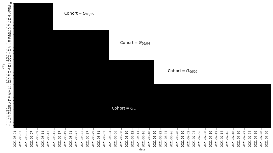

mkt_data_cohorts_w = mkt_data_cohorts.query("region=='W'")
mkt_data_cohorts_w.head()

	date	city	region	cohort	treated	tau	downloads	post
0	2021-05-01	1	W	2021-06-20	1	0.0	27.0	0
1	2021-05-02	1	W	2021-06-20	1	0.0	28.0	0
2	2021-05-03	1	W	2021-06-20	1	0.0	28.0	0
3	2021-05-04	1	W	2021-06-20	1	0.0	26.0	0
4	2021-05-05	1	W	2021-06-20	1	0.0	28.0	0

fig, (ax1, ax2) = plt.subplots(2, 1, figsize=(15, 10))

plt_data = (
    mkt_data_cohorts_w.groupby(["date", "cohort"])[["downloads"]].mean().reset_index()
)


for color, cohort in zip(
    ["C0", "C1", "C2", "C3"],
    mkt_data_cohorts_w.query("cohort!='2100-01-01'")["cohort"].unique(),
):
    df_cohort = plt_data.query("cohort==@cohort")
    sns.lineplot(
        data=df_cohort,
        x="date",
        y="downloads",
        label=pd.to_datetime(cohort).strftime("%Y-%m-%d"),
        ax=ax1,
    )
    ax1.vlines(x=cohort, ymin=25, ymax=50, color=color, ls="dotted", lw=3)


sns.lineplot(
    data=plt_data.query("cohort=='2100-01-01'"),
    x="date",
    y="downloads",
    label="$\infty$",
    lw=4,
    ls="-.",
    ax=ax1,
)

ax1.legend()
ax1.set_title("Multiple Cohorts - West Region")
plt_data = (
    mkt_data_cohorts_w.assign(
        days_to_treatment=lambda d: (
            (pd.to_datetime(d["date"]) - pd.to_datetime(d["cohort"])).dt.days
        )
    )
    .groupby(["date", "cohort"])[["downloads", "days_to_treatment"]]
    .mean()
    .reset_index()
)


for color, cohort in zip(
    ["C0", "C1", "C2", "C3"],
    mkt_data_cohorts_w.query("cohort!='2100-01-01'")["cohort"].unique(),
):
    df_cohort = plt_data.query("cohort==@cohort")
    sns.lineplot(
        data=df_cohort,
        x="days_to_treatment",
        y="downloads",
        label=pd.to_datetime(cohort).strftime("%Y-%m-%d"),
        ax=ax2,
    )

ax2.vlines(x=0, ymin=25, ymax=50, color="black", ls="dotted", lw=3)

ax2.set_title("Multiple Cohorts (Aligned) - West Region")
ax2.legend()
plt.tight_layout()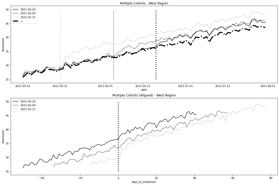

twfe_model = smf.ols(
    "downloads ~ treated:post + C(date) + C(city)", data=mkt_data_cohorts_w
).fit()

true_tau = mkt_data_cohorts_w.query("post==1&treated==1")["tau"].mean()

print("True Effect: ", true_tau)
print("Estimated ATT:", twfe_model.params["treated:post"])

True Effect:  2.2625252108176266
Estimated ATT: 1.7599504780633743

fig, (ax1, ax2) = plt.subplots(2, 1, figsize=(15, 10), sharex=True)

# fig, (ax1, ax2) = plt.subplots(2, 1, figsize=(10, 10))

cohort_erly = "2021-06-04"
cohort_late = "2021-06-20"

## Early vs Late
did_df = (
    mkt_data_cohorts_w.loc[lambda d: d["date"].astype(str) < cohort_late]
    .query(f"cohort=='{cohort_late}' | cohort=='{cohort_erly}'")
    .assign(
        treated=lambda d: (d["cohort"] == cohort_erly) * 1,
        post=lambda d: (d["date"].astype(str) >= cohort_erly) * 1,
    )
)

m = smf.ols("downloads ~ treated:post + C(date) + C(city)", data=did_df).fit()


# print("Estimated", m.params["treated:post"])
# print("True", did_df.query("post==1 & treated==1")["tau"].mean())

plt_data = (
    did_df.assign(installs_hat_0=lambda d: m.predict(d.assign(treated=0)))
    .groupby(["date", "cohort"])[["downloads", "post", "treated", "installs_hat_0"]]
    .mean()
    .reset_index()
)


sns.lineplot(data=plt_data, x="date", y="downloads", hue="cohort", ax=ax1)
sns.lineplot(
    data=plt_data.query("treated==1 & post==1"),
    x="date",
    y="installs_hat_0",
    ax=ax1,
    ls="-.",
    alpha=0.5,
    label="$\hat{Y}_0|T=1$",
)


ax1.vlines(pd.to_datetime(cohort_erly), 26, 38, ls="dashed")
ax1.legend()
ax1.set_title("Early vs Late")


# ## Late vs Early

did_df = (
    mkt_data_cohorts_w.loc[lambda d: d["date"].astype(str) > cohort_erly]
    .query(f"cohort=='{cohort_late}' | cohort=='{cohort_erly}'")
    .assign(
        treated=lambda d: (d["cohort"] == cohort_late) * 1,
        post=lambda d: (d["date"].astype(str) >= cohort_late) * 1,
    )
)

m = smf.ols("downloads ~ treated*post + C(date) + C(city)", data=did_df).fit()

# print("Estimated", m.params["treated:post"])
# print("True", did_df.query("post==1 & treated==1")["tau"].mean())


plt_data = (
    did_df.assign(installs_hat_0=lambda d: m.predict(d.assign(treated=0)))
    .groupby(["date", "cohort"])[["downloads", "post", "treated", "installs_hat_0"]]
    .mean()
    .reset_index()
)


sns.lineplot(data=plt_data, x="date", y="downloads", hue="cohort", ax=ax2)
sns.lineplot(
    data=plt_data.query("treated==1 & post==1"),
    x="date",
    y="installs_hat_0",
    ax=ax2,
    ls="-.",
    alpha=0.5,
    label="$\hat{Y}_0|T=1$",
)

ax2.vlines(pd.to_datetime("2021-06-20"), 32, 45, ls="dashed")
ax2.legend()
ax2.set_title("Late vs Early")

Text(0.5, 1.0, 'Late vs Early')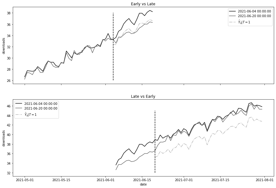

8.7.1 시간에 따른 이질적 효과

formula = "downloads ~ treated:post:C(cohort):C(date) + C(city)+C(date)"

twfe_model = smf.ols(formula, data=mkt_data_cohorts_w).fit()

df_pred = (
    mkt_data_cohorts_w.query("post==1 & treated==1")
    .assign(y_hat_0=lambda d: twfe_model.predict(d.assign(treated=0)))
    .assign(effect_hat=lambda d: d["downloads"] - d["y_hat_0"])
)

print("Number of param.:", len(twfe_model.params))
print("True Effect: ", df_pred["tau"].mean())
print("Pred. Effect: ", df_pred["effect_hat"].mean())

Number of param.: 510
True Effect:  2.2625252108176266
Pred. Effect:  2.259766144685074

formula = "downloads ~ treated:post:C(cohort):C(date) + C(city) + C(date)"

twfe_model = smf.ols(
    formula, data=mkt_data_cohorts_w.astype({"date": str, "cohort": str})
).fit()

effects = (
    twfe_model.params[twfe_model.params.index.str.contains("treated")]
    .reset_index()
    .rename(columns={0: "param"})
    .assign(cohort=lambda d: d["index"].str.extract(r"C\(cohort\)\[(.*)\]:"))
    .assign(date=lambda d: d["index"].str.extract(r":C\(date\)\[(.*)\]"))
    .assign(
        date=lambda d: pd.to_datetime(d["date"]),
        cohort=lambda d: pd.to_datetime(d["cohort"]),
    )
)

plt.figure(figsize=(10, 4))
sns.lineplot(data=effects, x="date", y="param", hue="cohort", palette="gray")
plt.xticks(rotation=45)
plt.ylabel("Estimated Effect")
plt.legend(fontsize=12)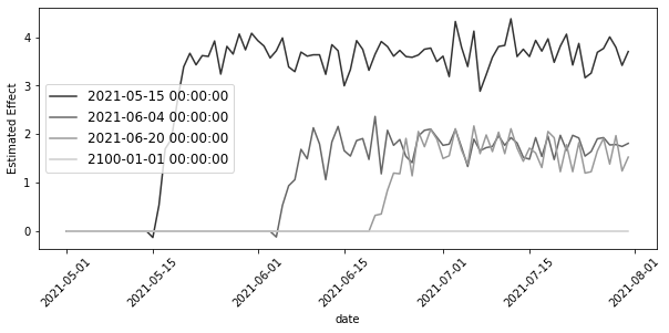

cohorts = sorted(mkt_data_cohorts_w["cohort"].unique())

treated_G = cohorts[:-1]
nvr_treated = cohorts[-1]


def did_g_vs_nvr_treated(
    df: pd.DataFrame,
    cohort: str,
    nvr_treated: str,
    cohort_col: str = "cohort",
    date_col: str = "date",
    y_col: str = "downloads",
):
    did_g = (
        df.loc[lambda d: (d[cohort_col] == cohort) | (d[cohort_col] == nvr_treated)]
        .assign(treated=lambda d: (d[cohort_col] == cohort) * 1)
        .assign(post=lambda d: (pd.to_datetime(d[date_col]) >= cohort) * 1)
    )

    att_g = smf.ols(f"{y_col} ~ treated*post", data=did_g).fit().params["treated:post"]
    size = len(did_g.query("treated==1 & post==1"))
    return {"att_g": att_g, "size": size}


atts = pd.DataFrame(
    [
        did_g_vs_nvr_treated(mkt_data_cohorts_w, cohort, nvr_treated)
        for cohort in treated_G
    ]
)

atts

	att_g	size
0	3.455535	702
1	1.659068	1044
2	1.573687	420

(atts["att_g"] * atts["size"]).sum() / atts["size"].sum()

2.2247467740558697

8.7.2 공변량

formula = """
downloads ~ treated:post:C(cohort):C(date)
+ C(date):C(region) + C(city) + C(date)"""

twfe_model = smf.ols(formula, data=mkt_data_cohorts).fit()

df_pred = (
    mkt_data_cohorts.query("post==1 & treated==1")
    .assign(y_hat_0=lambda d: twfe_model.predict(d.assign(treated=0)))
    .assign(effect_hat=lambda d: d["downloads"] - d["y_hat_0"])
)

print("Number of param.:", len(twfe_model.params))
print("True Effect: ", df_pred["tau"].mean())
print("Pred. Effect: ", df_pred["effect_hat"].mean())

Number of param.: 935
True Effect:  2.078397729895905
Pred. Effect:  2.0426262863584568

8.8 요약