5징 - 성향점수

import warnings

warnings.filterwarnings("ignore")

import pandas as pd
import numpy as np
import graphviz as gr
from matplotlib import style
import seaborn as sns
from matplotlib import pyplot as plt

style.use("ggplot")
import statsmodels.formula.api as smf
from cycler import cycler

color = ["0.2", "0.6", "1.0"]
default_cycler = cycler(color=color)
linestyle = ["-", "--", ":", "-."]
marker = ["o", "v", "d", "p"]


plt.rc("axes", prop_cycle=default_cycler)

5.1 관리자 교육의 효과

df = pd.read_csv("data/management_training.csv")
df.head()

	departament_id	intervention	engagement_score	tenure	n_of_reports	gender	role	last_engagement_score	department_score	department_size
0	76	1	0.277359	6	4	2	4	0.614261	0.224077	843
1	76	1	-0.449646	4	8	2	4	0.069636	0.224077	843
2	76	1	0.769703	6	4	2	4	0.866918	0.224077	843
3	76	1	-0.121763	6	4	2	4	0.029071	0.224077	843
4	76	1	1.526147	6	4	1	4	0.589857	0.224077	843

5.2 회귀분석과 보정

smf.ols("engagement_score ~ intervention", data=df).fit().summary().tables[1]

	coef	std err	t	P>|t|	[0.025	0.975]
Intercept	-0.2347	0.014	-16.619	0.000	-0.262	-0.207
intervention	0.4346	0.019	22.616	0.000	0.397	0.472

model = smf.ols(
    """engagement_score ~ intervention
+ tenure + last_engagement_score + department_score
+ n_of_reports + C(gender) + C(role)""",
    data=df,
).fit()

print("ATE:", model.params["intervention"])
print("95% CI:", model.conf_int().loc["intervention", :].values.T)

ATE: 0.2677908576676856
95% CI: [0.23357751 0.30200421]

5.3 성향점수

g = gr.Digraph(graph_attr={"rankdir": "LR"})
g.edge("T", "Y")
g.edge("X", "Y")
g.edge("X", "e(x)")
g.edge("e(x)", "T")

g

5.3.1 성향점수 추정

ps_model = smf.logit(
    """intervention ~
tenure + last_engagement_score + department_score
+ C(n_of_reports) + C(gender) + C(role)""",
    data=df,
).fit(disp=0)

data_ps = df.assign(
    propensity_score=ps_model.predict(df),
)

data_ps[["intervention", "engagement_score", "propensity_score"]].head()

	intervention	engagement_score	propensity_score
0	1	0.277359	0.596106
1	1	-0.449646	0.391138
2	1	0.769703	0.602578
3	1	-0.121763	0.580990
4	1	1.526147	0.619976

5.3.2 성향점수와 직교화

model = smf.ols(
    "engagement_score ~ intervention + propensity_score", data=data_ps
).fit()
model.params["intervention"]

0.26331267490277066

5.3.3 성향점수 매칭

from sklearn.neighbors import KNeighborsRegressor

T = "intervention"
X = "propensity_score"
Y = "engagement_score"

treated = data_ps.query(f"{T}==1")
untreated = data_ps.query(f"{T}==0")

mt0 = KNeighborsRegressor(n_neighbors=1).fit(untreated[[X]], untreated[Y])

mt1 = KNeighborsRegressor(n_neighbors=1).fit(treated[[X]], treated[Y])

predicted = pd.concat(
    [
        # find matches for the treated looking at the untreated knn model
        treated.assign(match=mt0.predict(treated[[X]])),
        # find matches for the untreated looking at the treated knn model
        untreated.assign(match=mt1.predict(untreated[[X]])),
    ]
)

predicted.head()

	departament_id	intervention	engagement_score	tenure	n_of_reports	gender	role	last_engagement_score	department_score	department_size	propensity_score	match
0	76	1	0.277359	6	4	2	4	0.614261	0.224077	843	0.596106	0.557680
1	76	1	-0.449646	4	8	2	4	0.069636	0.224077	843	0.391138	-0.952622
2	76	1	0.769703	6	4	2	4	0.866918	0.224077	843	0.602578	-0.618381
3	76	1	-0.121763	6	4	2	4	0.029071	0.224077	843	0.580990	-1.404962
4	76	1	1.526147	6	4	1	4	0.589857	0.224077	843	0.619976	0.000354

np.mean(
    (predicted[Y] - predicted["match"]) * predicted[T]
    + (predicted["match"] - predicted[Y]) * (1 - predicted[T])
)

0.28777443474045966

5.3.4 역확률 가중치

g_data = (
    data_ps.assign(
        weight=data_ps["intervention"] / data_ps["propensity_score"]
        + (1 - data_ps["intervention"]) / (1 - data_ps["propensity_score"]),
        propensity_score=data_ps["propensity_score"].round(2),
    )
    .groupby(["propensity_score", "intervention"])[["weight", "engagement_score"]]
    .mean()
    .reset_index()
)

plt.figure(figsize=(10, 4))
for t in [0, 1]:
    sns.scatterplot(
        data=g_data.query(f"intervention=={t}"),
        y="engagement_score",
        x="propensity_score",
        size="weight",
        sizes=(1, 100),
        color=color[t],
        legend=None,
        label=f"T={t}",
        marker=marker[t],
    )

plt.title("Inverse Probability of Treatment Weighting")
plt.legend()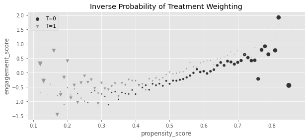

weight_t = 1 / data_ps.query("intervention==1")["propensity_score"]
weight_nt = 1 / (1 - data_ps.query("intervention==0")["propensity_score"])
t1 = data_ps.query("intervention==1")["engagement_score"]
t0 = data_ps.query("intervention==0")["engagement_score"]

y1 = sum(t1 * weight_t) / len(data_ps)
y0 = sum(t0 * weight_nt) / len(data_ps)

print("E[Y1]:", y1)
print("E[Y0]:", y0)
print("ATE", y1 - y0)

E[Y1]: 0.11656317232946772
E[Y0]: -0.1494155364781444
ATE 0.2659787088076121

np.mean(
    data_ps["engagement_score"]
    * (data_ps["intervention"] - data_ps["propensity_score"])
    / (data_ps["propensity_score"] * (1 - data_ps["propensity_score"]))
)

0.26597870880761226

5.3.5 역확률 가중치의 분산

from sklearn.linear_model import LogisticRegression
from patsy import dmatrix


# define function that computes the IPW estimator
def est_ate_with_ps(df, ps_formula, T, Y):
    X = dmatrix(ps_formula, df)
    ps_model = LogisticRegression(penalty="none", max_iter=1000).fit(X, df[T])
    ps = ps_model.predict_proba(X)[:, 1]

    # compute the ATE
    return np.mean((df[T] - ps) / (ps * (1 - ps)) * df[Y])

formula = """tenure + last_engagement_score + department_score
+ C(n_of_reports) + C(gender) + C(role)"""
T = "intervention"
Y = "engagement_score"

est_ate_with_ps(df, formula, T, Y)

0.2659755621752663

from joblib import Parallel, delayed  # for parallel processing


def bootstrap(data, est_fn, rounds=200, seed=123, pcts=[2.5, 97.5]):
    np.random.seed(seed)

    stats = Parallel(n_jobs=4)(
        delayed(est_fn)(data.sample(frac=1, replace=True)) for _ in range(rounds)
    )

    return np.percentile(stats, pcts)

from toolz import partial

print(f"ATE: {est_ate_with_ps(df, formula, T, Y)}")

est_fn = partial(est_ate_with_ps, ps_formula=formula, T=T, Y=Y)
print("95% C.I.: ", bootstrap(df, est_fn))

ATE: 0.2659755621752663
95% C.I.:  [0.22654315 0.30072595]

5.3.6 안정된 성향점수 가중치

print("Original Sample Size", data_ps.shape[0])
print("Treated Pseudo-Population Sample Size", sum(weight_t))
print("Untreated Pseudo-Population Sample Size", sum(weight_nt))

Original Sample Size 10391
Treated Pseudo-Population Sample Size 10435.089079197916
Untreated Pseudo-Population Sample Size 10354.298899788304

p_of_t = data_ps["intervention"].mean()

t1 = data_ps.query("intervention==1")
t0 = data_ps.query("intervention==0")

weight_t_stable = p_of_t / t1["propensity_score"]
weight_nt_stable = (1 - p_of_t) / (1 - t0["propensity_score"])

print("Treat size:", len(t1))
print("W treat", sum(weight_t_stable))

print("Control size:", len(t0))
print("W treat", sum(weight_nt_stable))

Treat size: 5611
W treat 5634.807508745978
Control size: 4780
W treat 4763.116999421415

nt = len(t1)
nc = len(t0)

y1 = sum(t1["engagement_score"] * weight_t_stable) / nt
y0 = sum(t0["engagement_score"] * weight_nt_stable) / nc

print("ATE: ", y1 - y0)

ATE:  0.26597870880761176

5.3.7 유사 모집단

fig, (ax1, ax2) = plt.subplots(1, 2, figsize=(12, 5), sharex=True, sharey=True)

sns.histplot(
    data_ps.query("intervention==0")["propensity_score"],
    stat="probability",
    label="Not Treated",
    color="C0",
    bins=30,
    ax=ax1,
    alpha=0.5,
)
sns.histplot(
    data_ps.query("intervention==1")["propensity_score"],
    stat="probability",
    label="Treated",
    color="C2",
    alpha=0.5,
    bins=30,
    ax=ax1,
)
ax1.set_title("Propensity Distribution")

sns.histplot(
    data_ps.query("intervention==0").assign(w=weight_nt_stable),
    x="propensity_score",
    stat="probability",
    color="C0",
    weights="w",
    label="Non Treated",
    bins=30,
    ax=ax2,
    alpha=0.5,
)

sns.histplot(
    data_ps.query("intervention==1").assign(w=weight_t_stable),
    x="propensity_score",
    stat="probability",
    color="C2",
    weights="w",
    label="Treated",
    bins=30,
    alpha=0.5,
    ax=ax2,
)
ax2.set_title("Weighted Propensity Distribution")
plt.legend()

plt.tight_layout()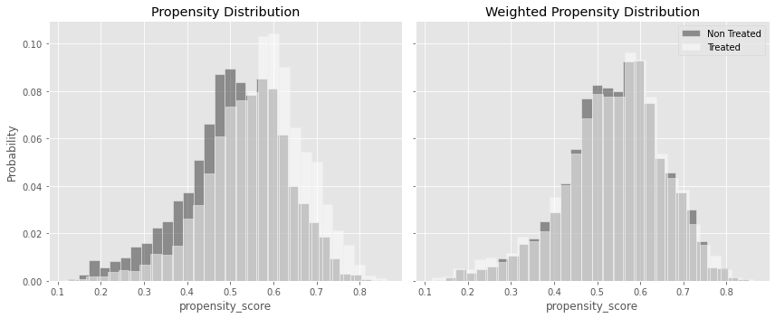

5.3.8 선택편향

5.3.9 편향-분산 트레이드오프

5.3.10 성향점수의 양수성 가정

np.random.seed(42)

n = 1000
x = np.random.normal(0, 1, n)
t = np.random.normal(x, 0.5, n) > 0

y0 = -x
y1 = y0 + t  # ate of 1

y = np.random.normal((1 - t) * y0 + t * y1, 0.2)

df_no_pos = pd.DataFrame(dict(x=x, t=t.astype(int), y=y))

df_no_pos.head()

	x	t	y
0	1.624345	1	-0.526442
1	-0.611756	0	0.659516
2	-0.528172	0	0.438549
3	-1.072969	0	0.950810
4	0.865408	1	-0.271397

ps_model_sim = smf.logit("""t ~ x""", data=df_no_pos).fit(disp=0)
df_no_pos_ps = df_no_pos.assign(ps=ps_model_sim.predict(df_no_pos))

ps = ps_model_sim.predict(df_no_pos)
w = df_no_pos["t"] * df_no_pos["t"].mean() / ps + (1 - df_no_pos["t"]) * (
    (1 - df_no_pos["t"].mean()) / (1 - ps)
)

fig, (ax1, ax2, ax3) = plt.subplots(1, 3, figsize=(16, 7))

sns.scatterplot(data=df_no_pos_ps.assign(w=w), x="x", y="y", hue="t", ax=ax1)
ax1.set_title("Original Data")

sns.histplot(
    df_no_pos_ps.query("t==0")["ps"],
    stat="probability",
    label="Non Treated",
    color="C0",
    bins=30,
    ax=ax2,
)
sns.histplot(
    df_no_pos_ps.query("t==1")["ps"],
    stat="probability",
    label="Treated",
    color="C1",
    alpha=0.5,
    bins=30,
    ax=ax2,
)
ax2.set_xlabel("e(x)")
ax2.legend()
ax2.set_title("Positivity Check")

sns.scatterplot(
    data=df_no_pos_ps.assign(**{"1/P(T=t)": w}),
    x="x",
    y="y",
    hue="t",
    ax=ax3,
    size="1/P(T=t)",
    sizes=(1, 100),
)
ax3.set_title("IPW Data")

plt.tight_layout()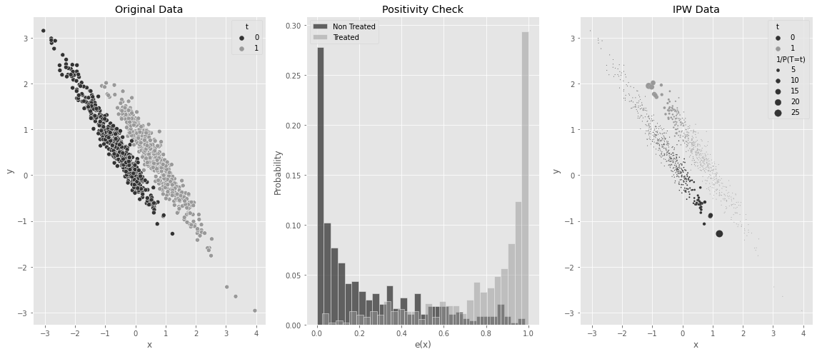

est_fn = partial(est_ate_with_ps, ps_formula="x", T="t", Y="y")
print("ATE:", est_fn(df_no_pos))
print("95% C.I.: ", bootstrap(df_no_pos, est_fn))

ATE: 0.6478011810615735
95% C.I.:  [0.41710504 0.88840195]

smf.ols("t ~ x + t", data=df_no_pos).fit().params["t"]

1.0

5.4 디자인 vs. 모델 기반 식별

5.5 이중 강건 추정

from sklearn.linear_model import LinearRegression


def doubly_robust(df, formula, T, Y):
    X = dmatrix(formula, df)

    ps_model = LogisticRegression(penalty="none", max_iter=1000).fit(X, df[T])
    ps = ps_model.predict_proba(X)[:, 1]

    m0 = LinearRegression().fit(X[df[T] == 0, :], df.query(f"{T}==0")[Y])
    m1 = LinearRegression().fit(X[df[T] == 1, :], df.query(f"{T}==1")[Y])

    m0_hat = m0.predict(X)
    m1_hat = m1.predict(X)

    return np.mean(df[T] * (df[Y] - m1_hat) / ps + m1_hat) - np.mean(
        (1 - df[T]) * (df[Y] - m0_hat) / (1 - ps) + m0_hat
    )

formula = """tenure + last_engagement_score + department_score
+ C(n_of_reports) + C(gender) + C(role)"""
T = "intervention"
Y = "engagement_score"

print("DR ATE:", doubly_robust(df, formula, T, Y))

est_fn = partial(doubly_robust, formula=formula, T=T, Y=Y)
print("95% CI", bootstrap(df, est_fn))

DR ATE: 0.27115831057931455
95% CI [0.23012681 0.30524944]

5.5.1 처치 모델링이 쉬운 경우

np.random.seed(123)

n = 10000
x = np.random.beta(1, 1, n).round(2) * 2
e = 1 / (1 + np.exp(-(1 + 1.5 * x)))
t = np.random.binomial(1, e)

y1 = 1
y0 = 1 - 1 * x**3
y = t * (y1) + (1 - t) * y0 + np.random.normal(0, 1, n)

df_easy_t = pd.DataFrame(dict(y=y, x=x, t=t))

print("True ATE:", np.mean(y1 - y0))

True ATE: 2.0056243152

fig, (ax1, ax2) = plt.subplots(1, 2, figsize=(12, 5))

sns.scatterplot(
    data=(
        df_easy_t.assign(size=1)
        .groupby(["x"])
        .agg({"size": "sum", "t": "mean"})
        .reset_index()
    ),
    x="x",
    y="t",
    sizes=(1, 100),
    size="size",
    ax=ax1,
)
ax1.set_title("P(T|X)")

sns.scatterplot(
    data=(
        df_easy_t.assign(size=1)
        .groupby(["x", "t"])
        .agg({"size": "sum", "y": "mean"})
        .reset_index()
    ),
    x="x",
    y="y",
    hue="t",
    sizes=(1, 100),
    size="size",
    ax=ax2,
)

ax2.set_title("E[Y|X, T]")

h, l = ax2.get_legend_handles_labels()
plt.legend(h[0:3], l[0:3])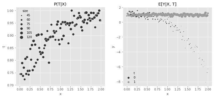

m0 = smf.ols("y~x", data=df_easy_t.query("t==0")).fit()
m1 = smf.ols("y~x", data=df_easy_t.query("t==1")).fit()
regr_ate = (m1.predict(df_easy_t) - m0.predict(df_easy_t)).mean()

print("Regression ATE:", regr_ate)

Regression ATE: 1.786678396833022

regr = smf.ols("y~x*t", data=df_easy_t).fit()

plt.figure(figsize=(10, 4))

sns.scatterplot(
    data=(
        df_easy_t.assign(count=1)
        .groupby(["x", "t"])
        .agg({"count": "sum", "y": "mean"})
        .reset_index()
    ),
    x="x",
    y="y",
    hue="t",
    sizes=(1, 100),
    size="count",
)
g = sns.lineplot(
    data=(
        df_easy_t.assign(pred=regr.fittedvalues)
        .groupby(["x", "t"])
        .mean()
        .reset_index()
    ),
    x="x",
    y="pred",
    hue="t",
    sizes=(1, 100),
)

h, l = g.get_legend_handles_labels()
plt.legend(h[0:3], l[0:3])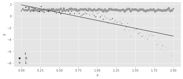

m = smf.ols("y~t*(x + np.power(x, 3))", data=df_easy_t).fit()
regr_ate = (m.predict(df_easy_t.assign(t=1)) - m.predict(df_easy_t.assign(t=0))).mean()

print("Regression ATE:", regr_ate)

Regression ATE: 1.9970999747190072

est_fn = partial(est_ate_with_ps, ps_formula="x", T="t", Y="y")
print("Propensity Score ATE:", est_fn(df_easy_t))
print("95% CI", bootstrap(df_easy_t, est_fn))

Propensity Score ATE: 2.002350388474011
95% CI [1.80802227 2.22565667]

est_fn = partial(doubly_robust, formula="x", T="t", Y="y")
print("DR ATE:", est_fn(df_easy_t))
print("95% CI", bootstrap(df_easy_t, est_fn))

DR ATE: 2.001617934263116
95% CI [1.87088771 2.145382  ]

5.5.2 결과 모델링이 쉬운 경우

np.random.seed(123)

n = 10000
x = np.random.beta(1, 1, n).round(2) * 2
e = 1 / (1 + np.exp(-(2 * x - x**3)))
t = np.random.binomial(1, e)

y1 = x
y0 = y1 + 1  # ate of -1
y = t * (y1) + (1 - t) * y0 + np.random.normal(0, 1, n)

df_easy_y = pd.DataFrame(dict(y=y, x=x, t=t))

print("True ATE:", np.mean(y1 - y0))

True ATE: -1.0

The same kind of plot from before can be used to show the complex functional form for \(P(T|X)\) and the simplicity of \(E[Y_t|X]\).

fig, (ax1, ax2) = plt.subplots(1, 2, figsize=(12, 5))

sns.scatterplot(
    data=(
        df_easy_y.assign(size=1)
        .groupby(["x"])
        .agg({"size": "sum", "t": "mean"})
        .reset_index()
    ),
    x="x",
    y="t",
    sizes=(1, 100),
    size="size",
    ax=ax1,
    legend=None,
)
sns.scatterplot(
    data=(
        df_easy_y.assign(size=1)
        .groupby(["x", "t"])
        .agg({"size": "sum", "y": "mean"})
        .reset_index()
    ),
    x="x",
    y="y",
    hue="t",
    sizes=(1, 100),
    size="size",
    ax=ax2,
)
ax1.set_title("P(T|X)")
ax2.set_title("E[Y|X, T]")

plt.legend(bbox_to_anchor=(1.05, 1), loc=2, borderaxespad=0.0)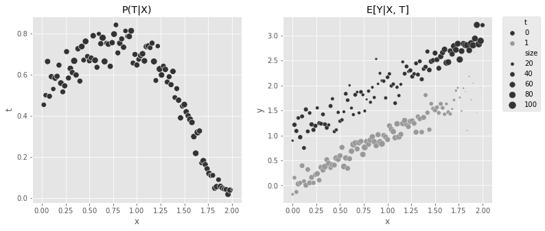

est_fn = partial(est_ate_with_ps, ps_formula="x", T="t", Y="y")
print("Propensity Score ATE:", est_fn(df_easy_y))
print("95% CI", bootstrap(df_easy_y, est_fn))

Propensity Score ATE: -1.1042900278680896
95% CI [-1.14326893 -1.06576358]

m0 = smf.ols("y~x", data=df_easy_y.query("t==0")).fit()
m1 = smf.ols("y~x", data=df_easy_y.query("t==1")).fit()
regr_ate = (m1.predict(df_easy_y) - m0.predict(df_easy_y)).mean()

print("Regression ATE:", regr_ate)

Regression ATE: -1.0008783612504342

est_fn = partial(doubly_robust, formula="x", T="t", Y="y")
print("DR ATE:", est_fn(df_easy_y))
print("95% CI", bootstrap(df_easy_y, est_fn))

DR ATE: -1.0028459347805823
95% CI [-1.04156952 -0.96353366]

5.6 연속형 처치에서의 일반화 성향점수

df_cont_t = pd.read_csv("../data/interest_rate.csv")

df_cont_t.head()

	ml_1	ml_2	interest	duration
0	0.392938	0.326285	7.1	12.0
1	-0.427721	0.679573	5.6	17.0
2	-0.546297	0.647309	11.1	12.0
3	0.102630	-0.264776	7.2	18.0
4	0.438938	-0.648818	9.5	19.0

m_naive = smf.ols("duration ~ interest", data=df_cont_t).fit()
m_naive.summary().tables[1]

	coef	std err	t	P>|t|	[0.025	0.975]
Intercept	14.5033	0.226	64.283	0.000	14.061	14.946
interest	0.3393	0.029	11.697	0.000	0.282	0.396

model_t = smf.ols("interest~ml_1+ml_2", data=df_cont_t).fit()

def conditional_density(x, mean, std):
    denom = std * np.sqrt(2 * np.pi)
    num = np.exp(-((1 / 2) * ((x - mean) / std) ** 2))
    return (num / denom).ravel()


gps = conditional_density(
    df_cont_t["interest"], model_t.fittedvalues, np.std(model_t.resid)
)
gps

array([0.1989118 , 0.14524168, 0.03338421, ..., 0.07339096, 0.19365006,
       0.15732008])

from scipy.stats import norm

gps = norm(loc=model_t.fittedvalues, scale=np.std(model_t.resid)).pdf(
    df_cont_t["interest"]
)
gps

array([0.1989118 , 0.14524168, 0.03338421, ..., 0.07339096, 0.19365006,
       0.15732008])

노트Beyond the Normal

If the treatment follows another distribution other than the normal, you can use generalized linear models (glm) to fit it. For example, if \(T\) was assigned according to a Poisson distribution, you could build the GPS weights with something like the following code

import statsmodels.api as sm
from scipy.stats import poisson
 
mt = smf.glm("t~x1+x2",
             data=df, family=sm.families.Poisson()).fit()
 
gps = poisson(mu=m_pois.fittedvalues).pmf(df["t"])
 
w = 1/gps

Using the inverse of the GPS as weights in a regression model can adjust for the bias. You can see that now you’ll find a negative effect of interest on duration, which makes more business sense.

final_model = smf.wls("duration~interest", data=df_cont_t, weights=1 / gps).fit()

final_model.params["interest"]

-0.6673977919925854

np.random.seed(42)
sample = df_cont_t.sample(2000)


model_ex = smf.ols("interest~ml_1", data=sample).fit()
gps_ex = norm(loc=model_ex.fittedvalues, scale=np.std(model_ex.resid)).pdf(
    sample["interest"]
)

w_ex = 1 / gps_ex

m = smf.ols("duration~interest", data=sample).fit()

fig, (ax1, ax2, ax3) = plt.subplots(1, 3, figsize=(16, 6))

sns.scatterplot(
    data=sample, x="interest", y="duration", alpha=1, ax=ax1, hue="ml_1", palette="gray"
)
ax1.plot(sample["interest"], m.fittedvalues)

ax1.set_ylabel("Duration")
ax1.set_xlabel("Interest")
ax1.set_title("Original Data")
sns.scatterplot(
    data=sample.assign(w=w_ex),
    x="ml_1",
    y="interest",
    size="w",
    sizes=(1, 200),
    alpha=0.5,
    ax=ax2,
)
ax2.plot(sample["ml_1"], model_ex.fittedvalues)
ax2.set_ylabel("Interest")
ax2.set_xlabel("ML-1")
ax2.set_title("Weights")


m = smf.wls("duration~interest", data=sample, weights=w_ex).fit()

sns.scatterplot(
    data=sample.assign(w=w_ex),
    x="interest",
    y="duration",
    size="w",
    sizes=(1, 200),
    alpha=1,
    ax=ax3,
    hue="ml_1",
    legend=None,
    palette="gray",
)
ax3.plot(sample["interest"], m.fittedvalues)
ax3.set_ylabel("Duration")
ax3.set_xlabel("Interest")
ax3.set_title("Weighted Data")

plt.tight_layout()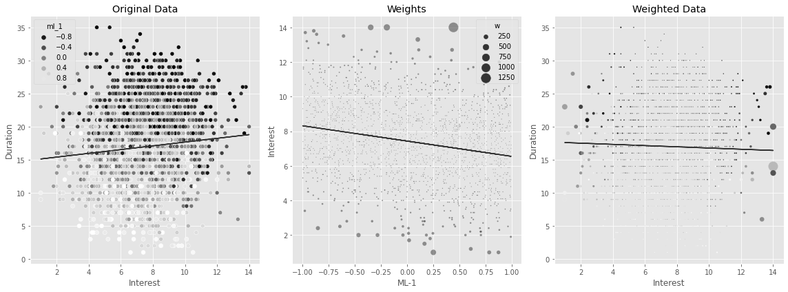

stabilizer = norm(
    loc=df_cont_t["interest"].mean(),
    scale=np.std(df_cont_t["interest"] - df_cont_t["interest"].mean()),
).pdf(df_cont_t["interest"])

gipw = stabilizer / gps

print("Original Sample Size:", len(df_cont_t))
print("Effective Stable Weights Sample Size:", sum(gipw))

Original Sample Size: 10000
Effective Stable Weights Sample Size: 9988.19595174861

np.random.seed(42)
sample = df_cont_t.sample(2000)

fig, (ax1, ax2, ax3) = plt.subplots(1, 3, figsize=(16, 6))

model_ex = smf.ols("interest~ml_1", data=sample).fit()
gps_ex = norm(loc=model_ex.fittedvalues, scale=np.std(model_ex.resid)).pdf(
    sample["interest"]
)
stabilizer_ex = norm(
    loc=sample["interest"].mean(),
    scale=np.std(sample["interest"] - sample["interest"].mean()),
).pdf(sample["interest"])


w_ex = stabilizer_ex / gps_ex

m = smf.ols("duration~interest", data=sample).fit()

sns.scatterplot(
    data=sample, x="interest", y="duration", alpha=1, ax=ax1, hue="ml_1", palette="gray"
)
ax1.plot(sample["interest"], m.fittedvalues, lw=3)
ax1.set_ylabel("Duration")
ax1.set_xlabel("Interest")
ax1.set_title("Original Data")
sns.scatterplot(
    data=sample.assign(w=w_ex),
    x="ml_1",
    y="interest",
    size="w",
    sizes=(1, 100),
    alpha=0.5,
    ax=ax2,
)

ax2.plot(sample["ml_1"], model_ex.fittedvalues, label="E[t|x]", lw=3)

ax2.hlines(sample["interest"].mean(), -1, 1, label="E[t]", color="C2", lw=3)
ax2.set_ylabel("Interest")
ax2.set_xlabel("ML-1")
ax2.set_title("Weights")

h, l = ax2.get_legend_handles_labels()
ax2.legend(
    h[5:],
    l[5:],
)

m = smf.wls("duration~interest", data=sample, weights=w_ex).fit()

sns.scatterplot(
    data=sample.assign(w=w_ex),
    x="interest",
    y="duration",
    size="w",
    sizes=(1, 100),
    alpha=1,
    ax=ax3,
    hue="ml_1",
    legend=None,
    palette="gray",
)
ax3.plot(sample["interest"], m.fittedvalues, lw=3)
ax3.set_ylabel("Duration")
ax3.set_xlabel("Interest")
ax3.set_title("Weighted Data")

Text(0.5, 1.0, 'Weighted Data')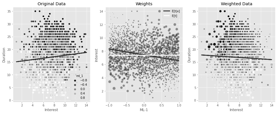

final_model = smf.wls("duration ~ interest", data=df_cont_t, weights=gipw).fit()

final_model.params["interest"]

-0.7787046278134069

def gps_normal_ate(df, formula, T, Y, stable=True):
    mt = smf.ols(f"{T}~" + formula, data=df).fit()
    gps = norm(loc=mt.fittedvalues, scale=np.std(mt.resid)).pdf(df[T])
    stabilizer = norm(loc=df[T].mean(), scale=np.std(df[T] - df[T].mean())).pdf(df[T])

    if stable:
        return smf.wls(f"{Y}~{T}", data=df, weights=stabilizer / gps).fit().params[T]
    else:
        return smf.wls(f"{Y}~{T}", data=df, weights=1 / gps).fit().params[T]


print(
    "95% CI, non-stable: ",
    bootstrap(
        df_cont_t,
        partial(
            gps_normal_ate,
            formula="ml_1 + ml_2",
            T="interest",
            Y="duration",
            stable=False,
        ),
    ),
)
print(
    "95% CI, stable: ",
    bootstrap(
        df_cont_t,
        partial(gps_normal_ate, formula="ml_1 + ml_2", T="interest", Y="duration"),
    ),
)

95% CI, non-stable:  [-0.81074164 -0.52605933]
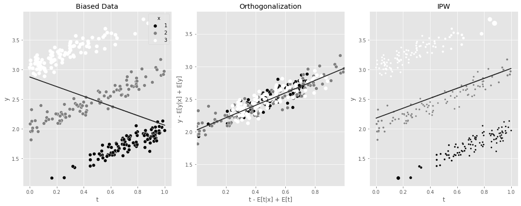
95% CI, stable:  [-0.85834311 -0.71001914]

5.7 요약

np.random.seed(42)

n = 100

df1 = pd.DataFrame(
    dict(
        x=1,
        t=np.random.beta(2.5, 1, n),
    )
).assign(y=lambda d: np.random.normal(d["x"] + d["t"], 0.1))

df2 = pd.DataFrame(
    dict(
        x=2,
        t=np.random.beta(1, 1, n),
    )
).assign(y=lambda d: np.random.normal(d["x"] + d["t"], 0.1))

df3 = pd.DataFrame(
    dict(
        x=3,
        t=np.random.beta(1, 2.5, n),
    )
).assign(y=lambda d: np.random.normal(d["x"] + d["t"], 0.1))


df_example = pd.concat([df1, df2, df3])

fig, (ax1, ax2, ax3) = plt.subplots(1, 3, figsize=(15, 6))

m = smf.ols("y~t", data=df_example).fit()
sns.scatterplot(data=df_example, x="t", y="y", hue="x", s=50, ax=ax1, palette="gray")
ax1.plot(df_example["t"], m.fittedvalues)
ax1.set_title("Biased Data")

## Orthogonalization

mt = smf.ols("t~x", data=df_example).fit()
my = smf.ols("y~x", data=df_example).fit()

df_ex_res = df_example.assign(
    t_res=mt.resid + df_example["t"].mean(), y_res=my.resid + df_example["y"].mean()
)

m_final = smf.ols("y_res~t_res", data=df_ex_res).fit()
sns.scatterplot(
    data=df_ex_res,
    x="t_res",
    y="y_res",
    hue="x",
    s=50,
    ax=ax2,
    legend=None,
    palette="gray",
)
ax2.plot(df_ex_res["t_res"], m_final.fittedvalues)

ax2.set_ylim(df_example["y"].min(), df_example["y"].max())
ax2.set_xlim(df_example["t"].min(), df_example["t"].max())

ax2.set_ylabel("y - E[y|x] + E[y]")
ax2.set_xlabel("t - E[t|x] + E[t]")
ax2.set_title("Orthogonalization")


## IPW
gps_example = norm(loc=mt.fittedvalues, scale=np.std(mt.resid)).pdf(df_example["t"])
stabilizer_example = norm(
    loc=df_example["t"].mean(), scale=np.std(df_example["t"] - df_example["t"].mean())
).pdf(df_example["t"])


w_example = stabilizer_example / gps_example
mw = smf.wls("y~t", data=df_example, weights=w_example).fit()


sns.scatterplot(
    data=df_example.assign(w=w_example),
    x="t",
    y="y",
    hue="x",
    ax=ax3,
    size="w",
    legend=None,
    sizes=(11, 100),
    palette="gray",
)
ax3.plot(df_example["t"], mw.fittedvalues)
ax3.set_title("IPW")

plt.tight_layout()