import warnings

warnings.filterwarnings("ignore")

import pandas as pd
import numpy as np
import graphviz as gr
from matplotlib import style
import seaborn as sns
from matplotlib import pyplot as plt

style.use("ggplot")
import statsmodels.formula.api as smf
from cycler import cycler

default_cycler = cycler(color=["0.3", "0.5", "0.7", "0.5"])

color = ["0.3", "0.5", "0.7", "0.9"]
linestyle = ["-", "--", ":", "-."]
marker = ["o", "v", "d", "p"]

plt.rc("axes", prop_cycle=default_cycler)

gr.set_default_format("png");4장 - 유용한 선형회귀
4.1 선형회귀의 필요성
4.1.1 모델이 필요한 이유
g_risk = gr.Digraph(graph_attr={"rankdir": "LR"})

g_risk.edge("Risk", "X")
g_risk.edge("X", "Credit Limit")
g_risk.edge("X", "Default")
g_risk.edge("Credit Limit", "Default")

g_risk
4.1.2 A/B 테스트와 회귀분석
무작위 실험인 A/B 테스트 결과를 분석할 때도 선형회귀를 사용하면 더 정밀한 추정치를 얻을 수 있습니다.
data = pd.read_csv("../data/rec_ab_test.csv")
data.head()| recommender | age | tenure | watch_time | |
|---|---|---|---|---|
| 0 | challenger | 15 | 1 | 2.39 |
| 1 | challenger | 27 | 1 | 2.32 |
| 2 | benchmark | 17 | 0 | 2.74 |
| 3 | benchmark | 34 | 1 | 1.92 |
| 4 | benchmark | 14 | 1 | 2.47 |
result = smf.ols("watch_time ~ C(recommender)", data=data).fit()

result.summary().tables[1]| coef | std err | t | P>|t| | [0.025 | 0.975] | |
|---|---|---|---|---|---|---|
| Intercept | 2.0491 | 0.058 | 35.367 | 0.000 | 1.935 | 2.163 |
| C(recommender)[T.challenger] | 0.1427 | 0.095 | 1.501 | 0.134 | -0.044 | 0.330 |
(data.groupby("recommender")["watch_time"].mean())recommender
benchmark 2.049064
challenger 2.191750
Name: watch_time, dtype: float644.1.3 회귀분석을 통한 보정
관측 데이터에서 발생할 수 있는 교란 요인들을 회귀 모델에 포함시켜 통제함으로써 인과 관계에 더 가까운 결과를 얻습니다.
risk_data = pd.read_csv("../data/risk_data.csv")

risk_data.head()| wage | educ | exper | married | credit_score1 | credit_score2 | credit_limit | default | |
|---|---|---|---|---|---|---|---|---|
| 0 | 950.0 | 11 | 16 | 1 | 500.0 | 518.0 | 3200.0 | 0 |
| 1 | 780.0 | 11 | 7 | 1 | 414.0 | 429.0 | 1700.0 | 0 |
| 2 | 1230.0 | 14 | 9 | 1 | 586.0 | 571.0 | 4200.0 | 0 |
| 3 | 1040.0 | 15 | 8 | 1 | 379.0 | 411.0 | 1500.0 | 0 |
| 4 | 1000.0 | 16 | 1 | 1 | 379.0 | 518.0 | 1800.0 | 0 |
model = smf.ols("default ~ credit_limit", data=risk_data).fit()
model.summary().tables[1]| coef | std err | t | P>|t| | [0.025 | 0.975] | |
|---|---|---|---|---|---|---|
| Intercept | 0.2192 | 0.004 | 59.715 | 0.000 | 0.212 | 0.226 |
| credit_limit | -2.402e-05 | 1.16e-06 | -20.689 | 0.000 | -2.63e-05 | -2.17e-05 |
plt_df = (
    risk_data.assign(size=1)
    .groupby("credit_limit")
    .agg({"default": "mean", "size": sum})
    .reset_index()
    .assign(prediction=lambda d: model.predict(d))
)

plt.figure(figsize=(10, 4))

sns.scatterplot(data=plt_df, x="credit_limit", y="default", size="size", sizes=(1, 100))

plt.plot(plt_df["credit_limit"], plt_df["prediction"], color="C1")
plt.title("Default Rate by Credit Limit")
Text(0.5, 1.0, 'Default Rate by Credit Limit')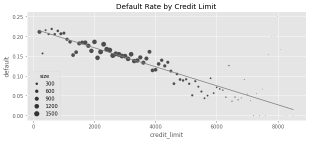
risk_data.groupby(["credit_score1", "credit_score2"]).size().head()credit_score1 credit_score2
34.0 339.0 1
500.0 1
52.0 518.0 1
69.0 214.0 1
357.0 1
dtype: int64formula = "default ~ credit_limit + wage+credit_score1+credit_score2"
model = smf.ols(formula, data=risk_data).fit()
model.summary().tables[1]| coef | std err | t | P>|t| | [0.025 | 0.975] | |
|---|---|---|---|---|---|---|
| Intercept | 0.4037 | 0.009 | 46.939 | 0.000 | 0.387 | 0.421 |
| credit_limit | 3.063e-06 | 1.54e-06 | 1.987 | 0.047 | 4.16e-08 | 6.08e-06 |
| wage | -8.822e-05 | 6.07e-06 | -14.541 | 0.000 | -0.000 | -7.63e-05 |
| credit_score1 | -4.175e-05 | 1.83e-05 | -2.278 | 0.023 | -7.77e-05 | -5.82e-06 |
| credit_score2 | -0.0003 | 1.52e-05 | -20.055 | 0.000 | -0.000 | -0.000 |
4.2 회귀분석 이론
X_cols = ["credit_limit", "wage", "credit_score1", "credit_score2"]
X = risk_data[X_cols].assign(intercep=1)
y = risk_data["default"]
def regress(y, X):
return np.linalg.inv(X.T.dot(X)).dot(X.T.dot(y))
beta = regress(y, X)
betaarray([ 3.06252773e-06, -8.82159125e-05, -4.17472814e-05, -3.03928359e-04,
4.03661277e-01])4.2.1 단순선형회귀
4.2.2 다중선형회귀
4.3 프리슈-워-로벨 정리와 직교화
formula = "default ~ credit_limit + wage+credit_score1+credit_score2"
model = smf.ols(formula, data=risk_data).fit()
model.summary().tables[1]| coef | std err | t | P>|t| | [0.025 | 0.975] | |
|---|---|---|---|---|---|---|
| Intercept | 0.4037 | 0.009 | 46.939 | 0.000 | 0.387 | 0.421 |
| credit_limit | 3.063e-06 | 1.54e-06 | 1.987 | 0.047 | 4.16e-08 | 6.08e-06 |
| wage | -8.822e-05 | 6.07e-06 | -14.541 | 0.000 | -0.000 | -7.63e-05 |
| credit_score1 | -4.175e-05 | 1.83e-05 | -2.278 | 0.023 | -7.77e-05 | -5.82e-06 |
| credit_score2 | -0.0003 | 1.52e-05 | -20.055 | 0.000 | -0.000 | -0.000 |
4.3.1 편향 제거 단계
plt_df = (
    risk_data.assign(size=1)
    .groupby("credit_limit")
    .agg({"default": "mean", "size": sum})
    .reset_index()
)

plt.figure(figsize=(10, 4))
sns.scatterplot(data=plt_df, x="credit_limit", y="default", size="size", sizes=(1, 100))


plt.title("Default Rate by Credit Limit")
Text(0.5, 1.0, 'Default Rate by Credit Limit')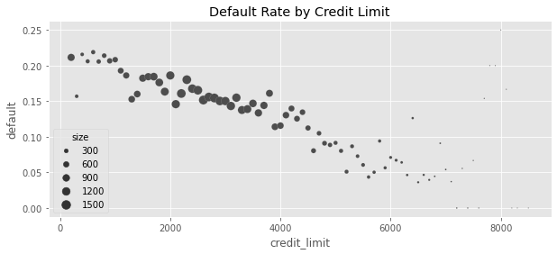
debiasing_model = smf.ols(
    "credit_limit ~ wage + credit_score1  + credit_score2", data=risk_data
).fit()

risk_data_deb = risk_data.assign(
    # for visualization, avg(T) is added to the residuals
    credit_limit_res=(debiasing_model.resid + risk_data["credit_limit"].mean())
)
model_w_deb_data = smf.ols("default ~ credit_limit_res", data=risk_data_deb).fit()
model_w_deb_data.summary().tables[1]| coef | std err | t | P>|t| | [0.025 | 0.975] | |
|---|---|---|---|---|---|---|
| Intercept | 0.1421 | 0.005 | 30.001 | 0.000 | 0.133 | 0.151 |
| credit_limit_res | 3.063e-06 | 1.56e-06 | 1.957 | 0.050 | -4.29e-09 | 6.13e-06 |
plt_df = (
    risk_data_deb.assign(size=1)
    .assign(credit_limit_res=lambda d: d["credit_limit_res"].round(-2))
    .groupby("credit_limit_res")
    .agg({"default": "mean", "size": sum})
    .query("size>30")
    .reset_index()
)

plt.figure(figsize=(10, 4))
sns.scatterplot(
    data=plt_df, x="credit_limit_res", y="default", size="size", sizes=(1, 100)
)

plt.title("Default Rate by Debiased Credit Limit")
Text(0.5, 1.0, 'Default Rate by Debiased Credit Limit')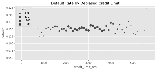
4.3.2 잡음 제거 단계
denoising_model = smf.ols(
    "default ~ wage + credit_score1  + credit_score2", data=risk_data_deb
).fit()

risk_data_denoise = risk_data_deb.assign(
    default_res=denoising_model.resid + risk_data_deb["default"].mean()
)
4.3.3 회귀 추정량의 표준오차
model_se = smf.ols(
    "default ~ wage + credit_score1  + credit_score2", data=risk_data
).fit()

print("SE regression:", model_se.bse["wage"])


model_wage_aux = smf.ols("wage ~ credit_score1 + credit_score2", data=risk_data).fit()

# subtract the degrees of freedom - 4 model parameters - from N.
se_formula = np.std(model_se.resid) / (
    np.std(model_wage_aux.resid) * np.sqrt(len(risk_data) - 4)
)

print("SE formula:   ", se_formula)
SE regression: 5.364242347548197e-06
SE formula: 5.364242347548201e-064.3.4 최종 결과 모델
model_w_orthogonal = smf.ols(
    "default_res ~ credit_limit_res", data=risk_data_denoise
).fit()

model_w_orthogonal.summary().tables[1]| coef | std err | t | P>|t| | [0.025 | 0.975] | |
|---|---|---|---|---|---|---|
| Intercept | 0.1421 | 0.005 | 30.458 | 0.000 | 0.133 | 0.151 |
| credit_limit_res | 3.063e-06 | 1.54e-06 | 1.987 | 0.047 | 4.17e-08 | 6.08e-06 |
plt_df = (
    risk_data_denoise.assign(size=1)
    .assign(credit_limit_res=lambda d: d["credit_limit_res"].round(-2))
    .groupby("credit_limit_res")
    .agg({"default_res": "mean", "size": sum})
    .query("size>30")
    .reset_index()
    .assign(prediction=lambda d: model_w_orthogonal.predict(d))
)

plt.figure(figsize=(10, 4))
sns.scatterplot(
    data=plt_df, x="credit_limit_res", y="default_res", size="size", sizes=(1, 100)
)

plt.plot(plt_df["credit_limit_res"], plt_df["prediction"], c="C1")

plt.title("Denoised Default Rate by Debiased Credit Limit")
Text(0.5, 1.0, 'Denoised Default Rate by Debiased Credit Limit')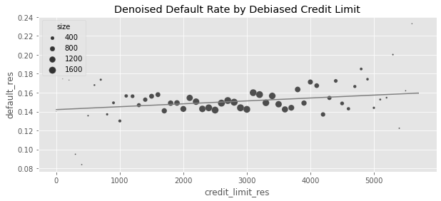
4.3.5 FWL 정리 요약
4.4 결과 모델으로서의 회귀분석
4.5 양수성과 외삽
np.random.seed(42)

n = 1000
x = np.random.normal(0, 1, n)
t = np.random.normal(x, 0.2, n) > 0

y0 = x
y1 = 1 + x

y = np.random.normal((1 - t) * y0 + t * y1, 0.2)

df_no_pos = pd.DataFrame(dict(x=x, t=t.astype(int), y=y))

fig, (ax1, ax2) = plt.subplots(1, 2, figsize=(12, 6), sharey=True)

sns.scatterplot(data=df_no_pos, x="x", y="y", hue="t", ax=ax1, label="treatment")

m0 = smf.ols("y~x", data=df_no_pos.query("t==0")).fit()
m1 = smf.ols("y~x", data=df_no_pos.query("t==1")).fit()

sns.lineplot(
    data=df_no_pos.assign(pred=m0.predict(df_no_pos)),
    x="x",
    y="pred",
    color="C0",
    ax=ax1,
)
sns.lineplot(
    data=df_no_pos.assign(pred=m1.predict(df_no_pos)),
    x="x",
    y="pred",
    color="C1",
    ax=ax1,
)
ax1.set_title("Dataset 1")

np.random.seed(42)

n = 1000
x = np.random.normal(0, 1, n)
t = np.random.binomial(1, 0.5, size=n)

y0 = x * (x < 0) + (x > 0) * 0
y1 = 1 + x

y = np.random.normal((1 - t) * y0 + t * y1, 0.2)

df_pos = pd.DataFrame(dict(x=x, t=t.astype(int), y=y))

sns.scatterplot(data=df_pos, x="x", hue="t", y="y", ax=ax2, label="treatment")

sns.lineplot(
    data=df_no_pos.assign(pred=m0.predict(df_pos)), x="x", y="pred", color="C0", ax=ax2
)
sns.lineplot(
    data=df_no_pos.assign(pred=m1.predict(df_pos)), x="x", y="pred", color="C1", ax=ax2
)
ax2.set_title("Dataset 2")
Text(0.5, 1.0, 'Dataset 2')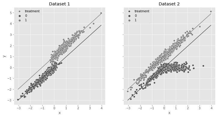
4.6 선형회귀에서의 비선형성
spend_data = pd.read_csv("../data/spend_data.csv")

spend_data.head()| wage | educ | exper | married | credit_score1 | credit_score2 | credit_limit | spend | |
|---|---|---|---|---|---|---|---|---|
| 0 | 950.0 | 11 | 16 | 1 | 500.0 | 518.0 | 3200.0 | 3848 |
| 1 | 780.0 | 11 | 7 | 1 | 414.0 | 429.0 | 1700.0 | 3144 |
| 2 | 1230.0 | 14 | 9 | 1 | 586.0 | 571.0 | 4200.0 | 4486 |
| 3 | 1040.0 | 15 | 8 | 1 | 379.0 | 411.0 | 1500.0 | 3327 |
| 4 | 1000.0 | 16 | 1 | 1 | 379.0 | 518.0 | 1800.0 | 3508 |
g_risk = gr.Digraph(graph_attr={"rankdir": "LR"})

g_risk.edge("Wage", "Credit Limit")
g_risk.edge("Wage", "Spend")
g_risk.edge("Credit Limit", "Spend")

g_risk
plt_df = (
    spend_data.assign(wage_group=lambda d: pd.IntervalIndex(pd.qcut(d["wage"], 5)).mid)
    .groupby(["wage_group", "credit_limit"])[["spend"]]
    .mean()
    .reset_index()
)

plt.figure(figsize=(10, 4))
sns.scatterplot(
    data=plt_df, x="credit_limit", y="spend", hue="wage_group", palette="gray"
)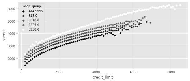
4.6.1 처치 선형화
plt_df = (
    spend_data
    # apply the sqrt function to the treatment
    .assign(credit_limit_sqrt=np.sqrt(spend_data["credit_limit"]))
    # create 5 wage binds for better vizualization
    .assign(wage_group=pd.IntervalIndex(pd.qcut(spend_data["wage"], 5)).mid)
    .groupby(["wage_group", "credit_limit_sqrt"])[["spend"]]
    .mean()
    .reset_index()
)

plt.figure(figsize=(10, 4))
sns.scatterplot(
    data=plt_df, x="credit_limit_sqrt", y="spend", palette="gray", hue="wage_group"
)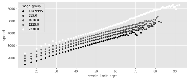
model_spend = smf.ols("spend ~ np.sqrt(credit_limit)", data=spend_data).fit()

model_spend.summary().tables[1]| coef | std err | t | P>|t| | [0.025 | 0.975] | |
|---|---|---|---|---|---|---|
| Intercept | 493.0044 | 6.501 | 75.832 | 0.000 | 480.262 | 505.747 |
| np.sqrt(credit_limit) | 63.2525 | 0.122 | 519.268 | 0.000 | 63.014 | 63.491 |
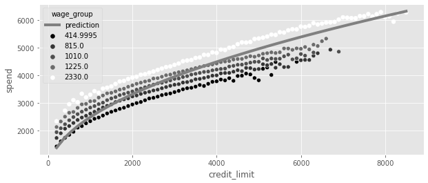
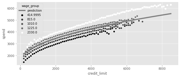
plt_df = (
    spend_data.assign(wage_group=lambda d: pd.IntervalIndex(pd.qcut(d["wage"], 5)).mid)
    .groupby(["wage_group", "credit_limit"])[["spend"]]
    .mean()
    .reset_index()
)

x = np.linspace(plt_df["credit_limit"].min(), plt_df["credit_limit"].max())

plt.figure(figsize=(10, 4))
plt.plot(
    x,
    model_spend.params[0] + model_spend.params[1] * np.sqrt(x),
    color="C1",
    label="prediction",
    lw=4,
)
plt.legend()
sns.scatterplot(
    data=plt_df, x="credit_limit", y="spend", palette="gray", hue="wage_group"
)
model_spend = smf.ols("spend ~ np.sqrt(credit_limit)+wage", data=spend_data).fit()

model_spend.summary().tables[1]| coef | std err | t | P>|t| | [0.025 | 0.975] | |
|---|---|---|---|---|---|---|
| Intercept | 383.5002 | 2.746 | 139.662 | 0.000 | 378.118 | 388.882 |
| np.sqrt(credit_limit) | 43.8504 | 0.065 | 672.633 | 0.000 | 43.723 | 43.978 |
| wage | 1.0459 | 0.002 | 481.875 | 0.000 | 1.042 | 1.050 |
4.6.2 비선형 FWL과 편향 제거
debias_spend_model = smf.ols("np.sqrt(credit_limit) ~ wage", data=spend_data).fit()
denoise_spend_model = smf.ols("spend ~ wage", data=spend_data).fit()


credit_limit_sqrt_deb = (
    debias_spend_model.resid + np.sqrt(spend_data["credit_limit"]).mean()
)
spend_den = denoise_spend_model.resid + spend_data["spend"].mean()


spend_data_deb = spend_data.assign(
    credit_limit_sqrt_deb=credit_limit_sqrt_deb, spend_den=spend_den
)

final_model = smf.ols("spend_den ~ credit_limit_sqrt_deb", data=spend_data_deb).fit()

final_model.summary().tables[1]| coef | std err | t | P>|t| | [0.025 | 0.975] | |
|---|---|---|---|---|---|---|
| Intercept | 1493.6990 | 3.435 | 434.818 | 0.000 | 1486.966 | 1500.432 |
| credit_limit_sqrt_deb | 43.8504 | 0.065 | 672.640 | 0.000 | 43.723 | 43.978 |
plt_df = (
    spend_data.assign(wage_group=lambda d: pd.IntervalIndex(pd.qcut(d["wage"], 5)).mid)
    .groupby(["wage_group", "credit_limit"])[["spend"]]
    .mean()
    .reset_index()
)

x = np.linspace(plt_df["credit_limit"].min(), plt_df["credit_limit"].max())

plt.figure(figsize=(10, 4))
plt.plot(
    x,
    (final_model.params[0] + final_model.params[1] * np.sqrt(x)),
    color="C1",
    label="prediction",
    lw=4,
)

plt.legend()

sns.scatterplot(
    data=plt_df, x="credit_limit", y="spend", palette="gray", hue="wage_group"
)
4.7 더미변수를 활용한 회귀분석
4.7.1 조건부 무작위 실험
risk_data_rnd = pd.read_csv("../data/risk_data_rnd.csv")
risk_data_rnd.head()| wage | educ | exper | married | credit_score1 | credit_score2 | credit_score1_buckets | credit_limit | default | |
|---|---|---|---|---|---|---|---|---|---|
| 0 | 890.0 | 11 | 16 | 1 | 490.0 | 500.0 | 400 | 5400.0 | 0 |
| 1 | 670.0 | 11 | 7 | 1 | 196.0 | 481.0 | 200 | 3800.0 | 0 |
| 2 | 1220.0 | 14 | 9 | 1 | 392.0 | 611.0 | 400 | 5800.0 | 0 |
| 3 | 1210.0 | 15 | 8 | 1 | 627.0 | 519.0 | 600 | 6500.0 | 0 |
| 4 | 900.0 | 16 | 1 | 1 | 275.0 | 519.0 | 200 | 2100.0 | 0 |
plt.figure(figsize=(15, 6))
sns.histplot(
    data=risk_data_rnd,
    x="credit_limit",
    hue="credit_score1_buckets",
    kde=True,
    palette="gray",
)
plt.title("Conditional random experiment")
Text(0.5, 1.0, 'Conditional random experiment')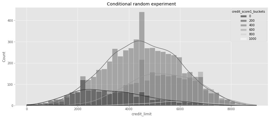
4.7.2 더미변수
model = smf.ols("default ~ credit_limit", data=risk_data_rnd).fit()
model.summary().tables[1]| coef | std err | t | P>|t| | [0.025 | 0.975] | |
|---|---|---|---|---|---|---|
| Intercept | 0.1369 | 0.009 | 15.081 | 0.000 | 0.119 | 0.155 |
| credit_limit | -9.344e-06 | 1.85e-06 | -5.048 | 0.000 | -1.3e-05 | -5.72e-06 |
pd.set_option("display.max_columns", 9)risk_data_dummies = risk_data_rnd.join(
pd.get_dummies(risk_data_rnd["credit_score1_buckets"], prefix="sb", drop_first=True)
)
risk_data_dummies.head()| wage | educ | exper | married | ... | sb_400 | sb_600 | sb_800 | sb_1000 | |
|---|---|---|---|---|---|---|---|---|---|
| 0 | 890.0 | 11 | 16 | 1 | ... | 1 | 0 | 0 | 0 |
| 1 | 670.0 | 11 | 7 | 1 | ... | 0 | 0 | 0 | 0 |
| 2 | 1220.0 | 14 | 9 | 1 | ... | 1 | 0 | 0 | 0 |
| 3 | 1210.0 | 15 | 8 | 1 | ... | 0 | 1 | 0 | 0 |
| 4 | 900.0 | 16 | 1 | 1 | ... | 0 | 0 | 0 | 0 |
5 rows × 14 columns
model = smf.ols(
    "default ~ credit_limit + sb_200+sb_400+sb_600+sb_800+sb_1000",
    data=risk_data_dummies,
).fit()

model.summary().tables[1]| coef | std err | t | P>|t| | [0.025 | 0.975] | |
|---|---|---|---|---|---|---|
| Intercept | 0.2253 | 0.056 | 4.000 | 0.000 | 0.115 | 0.336 |
| credit_limit | 4.652e-06 | 2.02e-06 | 2.305 | 0.021 | 6.97e-07 | 8.61e-06 |
| sb_200 | -0.0559 | 0.057 | -0.981 | 0.327 | -0.168 | 0.056 |
| sb_400 | -0.1442 | 0.057 | -2.538 | 0.011 | -0.256 | -0.033 |
| sb_600 | -0.2148 | 0.057 | -3.756 | 0.000 | -0.327 | -0.103 |
| sb_800 | -0.2489 | 0.060 | -4.181 | 0.000 | -0.366 | -0.132 |
| sb_1000 | -0.2541 | 0.094 | -2.715 | 0.007 | -0.438 | -0.071 |
model = smf.ols(
    "default ~ credit_limit + C(credit_score1_buckets)", data=risk_data_rnd
).fit()

model.summary().tables[1]| coef | std err | t | P>|t| | [0.025 | 0.975] | |
|---|---|---|---|---|---|---|
| Intercept | 0.2253 | 0.056 | 4.000 | 0.000 | 0.115 | 0.336 |
| C(credit_score1_buckets)[T.200] | -0.0559 | 0.057 | -0.981 | 0.327 | -0.168 | 0.056 |
| C(credit_score1_buckets)[T.400] | -0.1442 | 0.057 | -2.538 | 0.011 | -0.256 | -0.033 |
| C(credit_score1_buckets)[T.600] | -0.2148 | 0.057 | -3.756 | 0.000 | -0.327 | -0.103 |
| C(credit_score1_buckets)[T.800] | -0.2489 | 0.060 | -4.181 | 0.000 | -0.366 | -0.132 |
| C(credit_score1_buckets)[T.1000] | -0.2541 | 0.094 | -2.715 | 0.007 | -0.438 | -0.071 |
| credit_limit | 4.652e-06 | 2.02e-06 | 2.305 | 0.021 | 6.97e-07 | 8.61e-06 |
plt_df = (
    risk_data_rnd.assign(risk_prediction=model.fittedvalues)
    .groupby(["credit_limit", "credit_score1_buckets"])["risk_prediction"]
    .mean()
    .reset_index()
)

plt.figure(figsize=(10, 4))
sns.lineplot(
    data=plt_df,
    x="credit_limit",
    y="risk_prediction",
    hue="credit_score1_buckets",
    palette="gray",
)
plt.title("Fitted values by group")
plt.legend(loc="center left", bbox_to_anchor=(1, 0.5))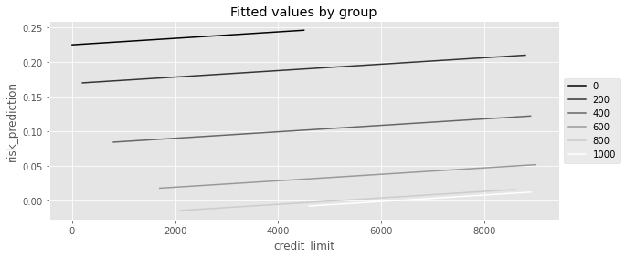
4.7.3 포화회귀모델
def regress(df, t, y):
    return smf.ols(f"{y}~{t}", data=df).fit().params[t]


effect_by_group = risk_data_rnd.groupby("credit_score1_buckets").apply(
    regress, y="default", t="credit_limit"
)
effect_by_group
credit_score1_buckets
0 -0.000071
200 0.000007
400 0.000005
600 0.000003
800 0.000002
1000 0.000000
dtype: float64group_size = risk_data_rnd.groupby("credit_score1_buckets").size()
ate = (effect_by_group * group_size).sum() / group_size.sum()
ate4.490445628748722e-06model = smf.ols(
"default ~ credit_limit * C(credit_score1_buckets)", data=risk_data_rnd
).fit()
model.summary().tables[1]| coef | std err | t | P>|t| | [0.025 | 0.975] | |
|---|---|---|---|---|---|---|
| Intercept | 0.3137 | 0.077 | 4.086 | 0.000 | 0.163 | 0.464 |
| C(credit_score1_buckets)[T.200] | -0.1521 | 0.079 | -1.926 | 0.054 | -0.307 | 0.003 |
| C(credit_score1_buckets)[T.400] | -0.2339 | 0.078 | -3.005 | 0.003 | -0.386 | -0.081 |
| C(credit_score1_buckets)[T.600] | -0.2957 | 0.080 | -3.690 | 0.000 | -0.453 | -0.139 |
| C(credit_score1_buckets)[T.800] | -0.3227 | 0.111 | -2.919 | 0.004 | -0.539 | -0.106 |
| C(credit_score1_buckets)[T.1000] | -0.3137 | 0.428 | -0.733 | 0.464 | -1.153 | 0.525 |
| credit_limit | -7.072e-05 | 4.45e-05 | -1.588 | 0.112 | -0.000 | 1.66e-05 |
| credit_limit:C(credit_score1_buckets)[T.200] | 7.769e-05 | 4.48e-05 | 1.734 | 0.083 | -1.01e-05 | 0.000 |
| credit_limit:C(credit_score1_buckets)[T.400] | 7.565e-05 | 4.46e-05 | 1.696 | 0.090 | -1.18e-05 | 0.000 |
| credit_limit:C(credit_score1_buckets)[T.600] | 7.398e-05 | 4.47e-05 | 1.655 | 0.098 | -1.37e-05 | 0.000 |
| credit_limit:C(credit_score1_buckets)[T.800] | 7.286e-05 | 4.65e-05 | 1.567 | 0.117 | -1.83e-05 | 0.000 |
| credit_limit:C(credit_score1_buckets)[T.1000] | 7.072e-05 | 8.05e-05 | 0.878 | 0.380 | -8.71e-05 | 0.000 |
(
    model.params[model.params.index.str.contains("credit_limit:")]
    + model.params["credit_limit"]
).round(9)
credit_limit:C(credit_score1_buckets)[T.200] 0.000007
credit_limit:C(credit_score1_buckets)[T.400] 0.000005
credit_limit:C(credit_score1_buckets)[T.600] 0.000003
credit_limit:C(credit_score1_buckets)[T.800] 0.000002
credit_limit:C(credit_score1_buckets)[T.1000] 0.000000
dtype: float64plt_df = (
risk_data_rnd.assign(risk_prediction=model.fittedvalues)
.groupby(["credit_limit", "credit_score1_buckets"])["risk_prediction"]
.mean()
.reset_index()
)
plt.figure(figsize=(10, 4))
sns.lineplot(
data=plt_df,
x="credit_limit",
y="risk_prediction",
hue="credit_score1_buckets",
palette="gray",
)
plt.title("Fitted values by group")
plt.legend(loc="center left", bbox_to_anchor=(1, 0.5))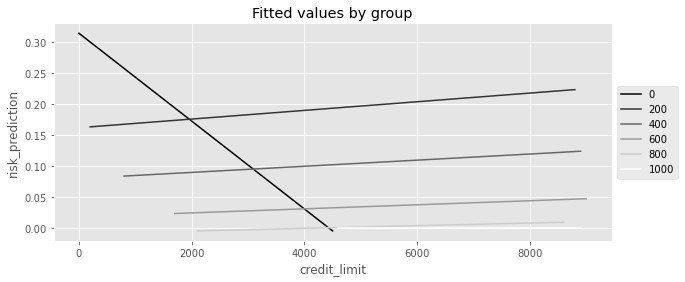
4.7.4 분산의 가중평균과 회귀분석
np.random.seed(123)

# std(t)=1
t1 = np.random.normal(0, 1, size=1000)
df1 = pd.DataFrame(
    dict(
        t=t1,
        y=1 * t1,  # ATE of 1
        g=1,
    )
)

# std(t)=2
t2 = np.random.normal(0, 2, size=500)
df2 = pd.DataFrame(
    dict(
        t=t2,
        y=2 * t2,  # ATE of 2
        g=2,
    )
)

df = pd.concat([df1, df2])
df.head()| t | y | g | |
|---|---|---|---|
| 0 | -1.085631 | -1.085631 | 1 |
| 1 | 0.997345 | 0.997345 | 1 |
| 2 | 0.282978 | 0.282978 | 1 |
| 3 | -1.506295 | -1.506295 | 1 |
| 4 | -0.578600 | -0.578600 | 1 |
effect_by_group = df.groupby("g").apply(regress, y="y", t="t")
ate = (effect_by_group * df.groupby("g").size()).sum() / df.groupby("g").size().sum()
ate1.333333333333333model = smf.ols("y ~ t + C(g)", data=df).fit()
model.paramsIntercept 0.024758
C(g)[T.2] 0.019860
t 1.625775
dtype: float644.7.5 평균 제거와 고정효과
model_deb = smf.ols("credit_limit ~ C(credit_score1_buckets)", data=risk_data_rnd).fit()
model_deb.summary().tables[1]| coef | std err | t | P>|t| | [0.025 | 0.975] | |
|---|---|---|---|---|---|---|
| Intercept | 1173.0769 | 278.994 | 4.205 | 0.000 | 626.193 | 1719.961 |
| C(credit_score1_buckets)[T.200] | 2195.4337 | 281.554 | 7.798 | 0.000 | 1643.530 | 2747.337 |
| C(credit_score1_buckets)[T.400] | 3402.3796 | 279.642 | 12.167 | 0.000 | 2854.224 | 3950.535 |
| C(credit_score1_buckets)[T.600] | 4191.3235 | 280.345 | 14.951 | 0.000 | 3641.790 | 4740.857 |
| C(credit_score1_buckets)[T.800] | 4639.5105 | 291.400 | 15.921 | 0.000 | 4068.309 | 5210.712 |
| C(credit_score1_buckets)[T.1000] | 5006.9231 | 461.255 | 10.855 | 0.000 | 4102.771 | 5911.076 |
risk_data_rnd.groupby("credit_score1_buckets")["credit_limit"].mean()credit_score1_buckets
0 1173.076923
200 3368.510638
400 4575.456498
600 5364.400448
800 5812.587413
1000 6180.000000
Name: credit_limit, dtype: float64risk_data_fe = risk_data_rnd.assign(
credit_limit_avg=lambda d: d.groupby("credit_score1_buckets")[
"credit_limit"
].transform("mean")
)model = smf.ols("default ~ I(credit_limit-credit_limit_avg)", data=risk_data_fe).fit()
model.summary().tables[1]| coef | std err | t | P>|t| | [0.025 | 0.975] | |
|---|---|---|---|---|---|---|
| Intercept | 0.0935 | 0.003 | 32.121 | 0.000 | 0.088 | 0.099 |
| I(credit_limit - credit_limit_avg) | 4.652e-06 | 2.05e-06 | 2.273 | 0.023 | 6.4e-07 | 8.66e-06 |
model = smf.ols("default ~ credit_limit + credit_limit_avg", data=risk_data_fe).fit()
model.summary().tables[1]| coef | std err | t | P>|t| | [0.025 | 0.975] | |
|---|---|---|---|---|---|---|
| Intercept | 0.4325 | 0.020 | 21.418 | 0.000 | 0.393 | 0.472 |
| credit_limit | 4.652e-06 | 2.02e-06 | 2.305 | 0.021 | 6.96e-07 | 8.61e-06 |
| credit_limit_avg | -7.763e-05 | 4.75e-06 | -16.334 | 0.000 | -8.69e-05 | -6.83e-05 |
4.8 누락 변수 편향
g = gr.Digraph(graph_attr={"rankdir": "LR"})


g.edge("Lines", "Default")
(g.edge("Wage", "Default"),)
g.edge("Wage", "Lines")


g
short_model = smf.ols("default ~ credit_limit", data=risk_data).fit()
short_model.params["credit_limit"]-2.401961992596885e-05long_model = smf.ols("default ~ credit_limit + wage", data=risk_data).fit()
omitted_model = smf.ols("wage ~ credit_limit", data=risk_data).fit()
(
long_model.params["credit_limit"]
+ long_model.params["wage"] * omitted_model.params["credit_limit"]
)-2.4019619925968762e-054.9 중립 통제변수
g = gr.Digraph(graph_attr={"rankdir": "LR"})

(g.edge("credit_score1_buckets", "Default"),)
(g.edge("credit_score1_buckets", "Lines"),)
(g.edge("credit_score2", "Default"),)
g.edge("Lines", "Default")

g
formula = "default~credit_limit+C(credit_score1_buckets)+credit_score2"
model = smf.ols(formula, data=risk_data_rnd).fit()
model.summary().tables[1]| coef | std err | t | P>|t| | [0.025 | 0.975] | |
|---|---|---|---|---|---|---|
| Intercept | 0.5576 | 0.055 | 10.132 | 0.000 | 0.450 | 0.665 |
| C(credit_score1_buckets)[T.200] | -0.0387 | 0.055 | -0.710 | 0.478 | -0.146 | 0.068 |
| C(credit_score1_buckets)[T.400] | -0.1032 | 0.054 | -1.898 | 0.058 | -0.210 | 0.003 |
| C(credit_score1_buckets)[T.600] | -0.1410 | 0.055 | -2.574 | 0.010 | -0.248 | -0.034 |
| C(credit_score1_buckets)[T.800] | -0.1161 | 0.057 | -2.031 | 0.042 | -0.228 | -0.004 |
| C(credit_score1_buckets)[T.1000] | -0.0430 | 0.090 | -0.479 | 0.632 | -0.219 | 0.133 |
| credit_limit | 4.928e-06 | 1.93e-06 | 2.551 | 0.011 | 1.14e-06 | 8.71e-06 |
| credit_score2 | -0.0007 | 2.34e-05 | -30.225 | 0.000 | -0.001 | -0.001 |
4.9.1 잡음 유발 통제변수
g = gr.Digraph(graph_attr={"rankdir": "LR"})


(g.edge("credit_score1_buckets", "Lines"),)
(g.edge("U", "Spend"),)
g.edge("Lines", "Spend")

g
spend_data_rnd = pd.read_csv("data/spend_data_rnd.csv")

model = smf.ols("spend ~ np.sqrt(credit_limit)", data=spend_data_rnd).fit()

model.summary().tables[1]| coef | std err | t | P>|t| | [0.025 | 0.975] | |
|---|---|---|---|---|---|---|
| Intercept | 2153.2154 | 218.600 | 9.850 | 0.000 | 1723.723 | 2582.708 |
| np.sqrt(credit_limit) | 16.2915 | 2.988 | 5.452 | 0.000 | 10.420 | 22.163 |
model = smf.ols(
    "spend~np.sqrt(credit_limit)+C(credit_score1_buckets)", data=spend_data_rnd
).fit()

model.summary().tables[1]| coef | std err | t | P>|t| | [0.025 | 0.975] | |
|---|---|---|---|---|---|---|
| Intercept | 2367.4867 | 556.273 | 4.256 | 0.000 | 1274.528 | 3460.446 |
| C(credit_score1_buckets)[T.200] | -144.7921 | 591.613 | -0.245 | 0.807 | -1307.185 | 1017.601 |
| C(credit_score1_buckets)[T.400] | -118.3923 | 565.364 | -0.209 | 0.834 | -1229.211 | 992.427 |
| C(credit_score1_buckets)[T.600] | -111.5738 | 570.471 | -0.196 | 0.845 | -1232.429 | 1009.281 |
| C(credit_score1_buckets)[T.800] | -89.7366 | 574.645 | -0.156 | 0.876 | -1218.791 | 1039.318 |
| C(credit_score1_buckets)[T.1000] | 363.8990 | 608.014 | 0.599 | 0.550 | -830.720 | 1558.518 |
| np.sqrt(credit_limit) | 14.5953 | 3.523 | 4.142 | 0.000 | 7.673 | 21.518 |
4.9.2 특성 선택: 편향-분산 트레이드오프
g = gr.Digraph(graph_attr={"rankdir": "LR"})


(g.edge("X1", "T", penwidth="5"),)
(g.edge("X2", "T", penwidth="3"),)
(g.edge("X3", "T", penwidth="1"),)

(g.edge("X1", "Y", penwidth="1"),)
(g.edge("X2", "Y", penwidth="3"),)
(g.edge("X3", "Y", penwidth="5"),)

(g.edge("T", "Y"),)

g
np.random.seed(123)

n = 100
(x1, x2, x3) = (np.random.normal(0, 1, n) for _ in range(3))
t = np.random.normal(10 * x1 + 5 * x2 + x3)

# ate = 0.05
y = np.random.normal(0.05 * t + x1 + 5 * x2 + 10 * x3, 5)
df = pd.DataFrame(dict(y=y, t=t, x1=x1, x2=x2, x3=x3))

smf.ols("y~t+x1+x2+x3", data=df).fit().summary().tables[1]| coef | std err | t | P>|t| | [0.025 | 0.975] | |
|---|---|---|---|---|---|---|
| Intercept | 0.2707 | 0.527 | 0.514 | 0.608 | -0.775 | 1.316 |
| t | 0.8664 | 0.607 | 1.427 | 0.157 | -0.339 | 2.072 |
| x1 | -7.0628 | 6.038 | -1.170 | 0.245 | -19.049 | 4.923 |
| x2 | 0.0143 | 3.128 | 0.005 | 0.996 | -6.195 | 6.224 |
| x3 | 9.6292 | 0.887 | 10.861 | 0.000 | 7.869 | 11.389 |
smf.ols("y~t+x2+x3", data=df).fit().summary().tables[1]| coef | std err | t | P>|t| | [0.025 | 0.975] | |
|---|---|---|---|---|---|---|
| Intercept | 0.1889 | 0.523 | 0.361 | 0.719 | -0.849 | 1.227 |
| t | 0.1585 | 0.046 | 3.410 | 0.001 | 0.066 | 0.251 |
| x2 | 3.6095 | 0.582 | 6.197 | 0.000 | 2.453 | 4.766 |
| x3 | 10.4549 | 0.537 | 19.453 | 0.000 | 9.388 | 11.522 |
4.10 요약
import graphviz as gr

g = gr.Digraph(format="png")

g.edge("Parent's Income", "Private")
g.edge("SAT", "Private")
g.edge("Ambition", "Private")
g.edge("...", "Private")

g.edge("Parent's Income", "Income")
g.edge("SAT", "Income")
g.edge("Ambition", "Income")
g.edge("...", "Income")

g.edge("Private", "Income")

g