| SMILES | ID | ChEMBL_ID | label | Mol | mw | logP | charge | |
|---|---|---|---|---|---|---|---|---|
| 0 | Cn1ccnc1Sc2ccc(cc2Cl)Nc3c4cc(c(cc4ncc3C#N)OCCC... | 168691 | CHEMBL318804 | Active |  |
565.099 | 5.49788 | 0 |
| 1 | C[C@@]12[C@@H]([C@@H](CC(O1)n3c4ccccc4c5c3c6n2... | 86358 | CHEMBL162 | Active |  |
466.541 | 4.35400 | 0 |
| 2 | Cc1cnc(nc1c2cc([nH]c2)C(=O)N[C@H](CO)c3cccc(c3... | 575087 | CHEMBL576683 | Active |  |
527.915 | 4.96202 | 0 |
| 3 | Cc1cnc(nc1c2cc([nH]c2)C(=O)N[C@H](CO)c3cccc(c3... | 575065 | CHEMBL571484 | Active |  |
491.935 | 4.36922 | 0 |
| 4 | Cc1cnc(nc1c2cc([nH]c2)C(=O)N[C@H](CO)c3cccc(c3... | 575047 | CHEMBL568937 | Active |  |
487.991 | 5.12922 | 0 |
Chapter 11: 특화된 예측 모델
이 장에서는 ERK2 활성 결합(ERK2 binding) 및 화학물질 라이브러리 필터링(filtering chemical libraries)과 같은 특정 과업을 수행하기 위한 고급 예측 모델에 대해 다룹니다.
ERK2 예측 모델 (ERK2 Predictive Models)
01: 예측 모델 구축 준비
예측 모델 구축을 위한 데이터셋 준비
첫 번째 단계로 ERK2 활성을 예측하는 그래프 합성곱 모델을 만들겠습니다. ERK2 활성(active) 화합물 모음과 비활성 유인(decoy) 화합물 모음을 분류하도록 모델을 학습시킬 것입니다. 활성 및 decoy 화합물은 DUD-E 데이터베이스로부터 가져왔습니다. 가장 정확한 모델을 구축하려면, 활성 화합물과 유사한 물성 분포(property distributions)를 지닌 유인 화합물들이 필요합니다. 만약 유인 화합물이 활성 화합물보다 평균적으로 분자량이 낮아서 이 특성이 차이가 난다면, 우리가 만든 분류기는 활성과 비활성이 아니라 단지 저분자량 화합물과 고분자량 화합물을 구별하도록 학습될 것입니다. 이는 실제 응용에서 매우 유용하지 않습니다.
따라서, 모델 학습 전 활성화합물과 유인 화합물의 계산 가능한 특성 몇 가지를 먼저 살펴보겠습니다. 신뢰할 수 있는 예측 모델을 구축하려면 활성 분자와 decoy의 특성이 전반적으로 유사하다는 점을 명확히 해야 합니다.
우선 필요한 라이브러리들을 임포트합니다.
이제 SMILES 파일을 Pandas 데이터프레임 형식으로 읽어들이고, RDKit 분자 객체를 데이터프레임에 추가할 수 있습니다.
데이터프레임에 화합물의 계산된 물성치들을 추가하는 함수를 정의하겠습니다.
이 함수를 활용하면 분자의 분자량(molecular weight), LogP, 그리고 형식 전하(formal charge)를 계산할 수 있습니다. 계산이 끝나면 활성 세트와 유인(decoy) 세트의 분포를 비교할 수 있습니다.
데이터프레임의 첫 몇 행을 확인해 올바르게 수행되었는지 확인합니다.
유인 화합물에 대해서도 똑같은 과정을 반복하겠습니다.
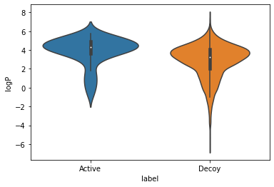
활성 세트와 유인 세트 모두에 대해 특성 계산이 완료되었으므로 두 그룹 간의 속성을 비교할 수 있습니다. 비교를 위해 바이올린 플롯(violin plots)을 사용하겠습니다. 바이올린 플롯은 박스플롯(boxplot)과 유사하지만 빈도 분포를 좌우 대칭으로 한눈에 보여줍니다. 기계학습 모델의 예측력을 높이려면 활성 데이터와 유인(decoy) 데이터 사이에 유사한 분포가 나타나는 것이 이상적입니다.

위 그림에서 두 세트의 분자량 분포가 대체로 동일하다는 것을 알 수 있습니다. 유인(decoy) 세트 쪽에 낮은 분자량 화합물이 더 많기는 하지만, 각 바이올린 플롯 중간에 표시된 상자로 볼 수 있는 분포의 중심값은 두 그래프 모두 비슷한 위치에 놓여 있습니다.
바이올린 플롯을 통해 LogP 분포 간 비슷한 비교도 가능합니다. 여기서도 유인(decoy) 그룹 하위권 범위에 화합물이 약간 더 포함되어 있으나 두 분포의 전반적 양상은 크게 다르지 않음을 확인할 수 있습니다.
마지막으로 두 화합물 집합의 분자 형식 전하(formal charges)를 살펴보겠습니다.
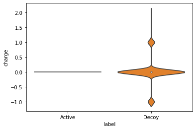
여기서 큰 차이가 보입니다. 활성 화합물 그룹은 모두 중성인데 일부 유인(decoy) 화합물들은 전하를 띠고 있습니다. 전체 분자 중 전하를 띠는 유인 화합물의 비율이 얼마나 될지 확인해 보겠습니다. 그러기 위해 전하를 띤 분자들만 따로 추출해 새로운 데이터프레임을 만듭니다.
Pandas 데이터프레임은 행(row)과 열(column)의 수를 나타내는 shape 속성을 가지고 있습니다. 즉, shape 속성의 첫 번째 요소(element[0])가 행의 수가 됩니다. 전하를 띤 분자 데이터프레임 행의 개수를 전체 유인(decoy) 데이터프레임 행 개수로 나누어 비율을 구해보겠습니다.
0.16175824175824177활성 화합물 그룹 중에는 전하를 띤 화합물이 하나도 없는데, 유인(decoy) 화합물의 무려 16%가 전하를 띠는 상태라는 것은 문제입니다. 분석해 본 결과 이유는 활성화합물에는 전하 상태 정보가 할당되지 않았고 비활성 화합물인 decoy 화합물 쪽에만 적용되었기 때문입니다. 두 그룹 간 통일성을 유지하기 위해 RDKit Cookbook에서 분자 전하를 중화(neutralize)시키는 기존 코드를 사용할 것입니다. 우선 전하를 중화시키는 RDKit 함수를 가져옵니다.
이제 유인(decoy) 화합물들의 SMILES, ID, 그리고 라벨(label) 값을 가지고 새로운 데이터프레임을 생성해줍니다.
새로운 데이터프레임이 준비되었으니 SMILES를 중성화된 상태를 나타내는 코드로 한 번 교체하겠습니다. NeutraliseCharges(전하 중화) 함수는 분자의 전하 중립 형태 SMILES 문자열과 분자가 실제로 변경되었는지를 알리는 논리 변수(boolean) 모델을 담아 2개 튜플 값으로 전달합니다. 여기서는 SMILES 정보만 필요하므로, 전달 요소 중 첫째 파트만을 발췌하여 사용할 것입니다.
SMILES 교체가 끝나면 데이터프레임 구조에 분자 파싱 정보를 추가 배치하고 관련 물성값 계산 작업을 추가로 이입할 겁니다.
수정이 끝난 신규 중성화 유인(decoy) 데이터프레임의 끝부분에 본래 지니고 있었던 오리지널 활성 데이터프레임 원본 데이터를 붙여 넣고 다시 박스플롯(box plot) 모델을 도출합니다.
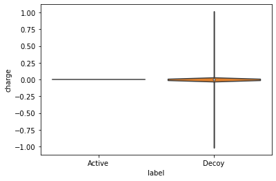
위 플롯 결과를 보면 decoy 데이터 세트에 전하를 띤 분자가 거의 없는 것으로 나타납니다. 위에서 전하를 띤 분자 데이터프레임을 추출했던 과정을 똑같이 적용해 남아 있는 전하 분자가 얼마나 있는지 알아낼 수 있습니다.
0.0026373626373626374처음 16%까지 미치던 전하 분자의 비율이 성공적으로 0.3%에 이르도록 줄어든 것을 볼 수 있습니다. 이제 활성 데이터세트와 유인 데이터세트가 아주 적절한 균형을 유지하고 있다고 신뢰할 수 있습니다.
이 데이터 세트를 DeepChem과 함께 구동시키려면 필수적으로 SMILES 정보 열, 화합물 명칭, 마지막으로 해당되는 각 화합물이 실질적인 활성치(1표기)을 갖는지 혹은 비활성치(0 표기)인지를 직접 가리키게 하여 이를 표식하는 정수 코드를 명기한 csv 포맷 파일 속으로 저장해야만 합니다.
| SMILES | ID | is_active | |
|---|---|---|---|
| 0 | Cn1ccnc1Sc2ccc(cc2Cl)Nc3c4cc(c(cc4ncc3C#N)OCCC... | 168691 | 1 |
| 1 | C[C@@]12[C@@H]([C@@H](CC(O1)n3c4ccccc4c5c3c6n2... | 86358 | 1 |
| 2 | Cc1cnc(nc1c2cc([nH]c2)C(=O)N[C@H](CO)c3cccc(c3... | 575087 | 1 |
| 3 | Cc1cnc(nc1c2cc([nH]c2)C(=O)N[C@H](CO)c3cccc(c3... | 575065 | 1 |
| 4 | Cc1cnc(nc1c2cc([nH]c2)C(=O)N[C@H](CO)c3cccc(c3... | 575047 | 1 |
마지막 단계로 기존 파일의 끝단에서 마무리된 새로운 통합 문서 데이터 combined_df 를 최종 csv 파일에 이식하여 담아내는 과정입니다. index=False 옵션을 활용함으로써 데이터 조립기인 Pandas 모듈이 csv 출력을 담당 시 인덱스 라벨들을 파일 앞쪽 열(column)에 무단 기재하는 현상을 차단할 수 있습니다.
02: 그래프 합성곱 신경망 활용
그래프 합성곱(Graph Convolution) 모델 학습
이제 적절한 형식으로 데이터를 준비했으므로, 이 데이터를 사용해 그래프 합성곱 모델을 학습시킬 수 있습니다. 먼저 필요한 라이브러리를 임포트해야 합니다.
이제 GraphConvModel을 생성하는 함수를 정의해 봅시다. 이 예제에서는 분류(classification) 모델을 생성할 것입니다. 모델을 나중에 다른 데이터셋에 적용할 예정이므로, 모델을 저장할 디렉토리를 만들어 두는 것이 좋습니다.
이제 방금 생성한 데이터셋을 읽어보겠습니다.
데이터셋이 로드되었으므로 모델을 구축해 봅시다. 모델 성능을 평가할 학습(train) 및 테스트(test) 세트를 생성합니다. 여기서는 RandomSplitter()를 사용합니다. DeepChem은 화학적 스캐폴드를 기준으로 분할하는 ScaffoldSplitter나, 데이터를 먼저 군집화한 후 서로 다른 군집이 학습/테스트 세트에 들어가도록 나누는 ButinaSplitter 등 다양한 분할기를 제공합니다.
데이터셋이 분할되었으니, 학습 세트로 모델을 학습시키고 검증(validation) 세트로 해당 모델을 테스트할 수 있습니다. 이 단계에서 몇 가지 평가지표(metrics)를 정의하여 모델의 성능을 평가할 수 있습니다. 이번 예제의 데이터셋은 불균형(unbalanced)합니다. 소수의 활성(active) 화합물과 다수의 비활성(inactive) 화합물로 구성되어 있죠. 이러한 차이를 고려하여 불균형 데이터셋에 맞는 평가지표를 사용해야 합니다. 이런 데이터셋에 적합한 평가지표 중 하나가 매튜스 상관계수(MCC, Matthews correlation coefficient)입니다.
모델 성능을 제대로 평가하기 위해 10-fold 교차 검증(cross validation)을 수행하겠습니다. 학습 세트로 모델을 학습시키고 검증 세트로 검증을 진행합니다.
WARNING:tensorflow:5 out of the last 292 calls to <function KerasModel._create_gradient_fn.<locals>.apply_gradient_for_batch at 0x7efdb4442158> triggered tf.function retracing. Tracing is expensive and the excessive number of tracings could be due to (1) creating @tf.function repeatedly in a loop, (2) passing tensors with different shapes, (3) passing Python objects instead of tensors. For (1), please define your @tf.function outside of the loop. For (2), @tf.function has experimental_relax_shapes=True option that relaxes argument shapes that can avoid unnecessary retracing. For (3), please refer to https://www.tensorflow.org/tutorials/customization/performance#python_or_tensor_args and https://www.tensorflow.org/api_docs/python/tf/function for more details.[0.5914454263139519, 0.9015009144980859, 0.7611553759655929, 0.9166857929681456, 0.7515870712054968, 0.8430723059543884, 0.7317218432848368, 0.6841835676310114, 0.781782969362093, 0.7676840845478065]
[0.5435391270264687, 0.8433069208152789, 0.7047972264664374, 0.8156105290325103, 0.8934523381859952, 0.9417724178034133, 0.7729109291165613, 0.7973563935758823, 0.4433162349439269, 0.701658436422957]학습 및 테스트 데이터에 대한 모델 성능을 시각화하기 위해 박스플롯(boxplot)을 그릴 수 있습니다.

모델 예측 결과를 시각화하는 것도 매우 유용합니다. 이를 위해 검증 세트에 대한 예측 값을 생성해 보겠습니다.
[array([0.99851984, 0.00148015], dtype=float32),
 array([9.9968302e-01, 3.1693748e-04], dtype=float32),
 array([0.99666446, 0.00333549], dtype=float32),
 array([0.47454447, 0.52545553], dtype=float32),
 array([0.9975573 , 0.00244266], dtype=float32),
 array([0.9974778 , 0.00252217], dtype=float32),
 array([0.9983169 , 0.00168311], dtype=float32),
 array([9.994553e-01, 5.447795e-04], dtype=float32),
 array([0.99608576, 0.00391427], dtype=float32),
 array([0.99847347, 0.00152652], dtype=float32),
 array([0.9897328 , 0.01026724], dtype=float32),
 array([0.99893624, 0.00106372], dtype=float32),
 array([0.99799097, 0.00200903], dtype=float32),
 array([0.9975101 , 0.00248989], dtype=float32),
 array([0.9977652 , 0.00223487], dtype=float32),
 array([0.997755  , 0.00224501], dtype=float32),
 array([9.9956113e-01, 4.3885410e-04], dtype=float32),
 array([9.9928027e-01, 7.1975554e-04], dtype=float32),
 array([0.9942093 , 0.00579075], dtype=float32),
 array([0.99854374, 0.00145632], dtype=float32),
 array([9.9970394e-01, 2.9598473e-04], dtype=float32),
 array([0.9923063 , 0.00769374], dtype=float32),
 array([0.99468684, 0.0053132 ], dtype=float32),
 array([0.9967669 , 0.00323309], dtype=float32),
 array([0.985803  , 0.01419694], dtype=float32),
 array([0.9965217 , 0.00347829], dtype=float32),
 array([9.9910057e-01, 8.9951378e-04], dtype=float32),
 array([0.9975655 , 0.00243455], dtype=float32),
 array([0.9977756 , 0.00222435], dtype=float32),
 array([0.99820924, 0.0017908 ], dtype=float32),
 array([0.99792504, 0.00207488], dtype=float32),
 array([9.9978548e-01, 2.1456773e-04], dtype=float32),
 array([0.99780065, 0.00219938], dtype=float32),
 array([0.99471384, 0.00528612], dtype=float32),
 array([0.9949008 , 0.00509917], dtype=float32),
 array([0.9431786 , 0.05682134], dtype=float32),
 array([0.9828377 , 0.01716235], dtype=float32),
 array([0.9966073 , 0.00339271], dtype=float32),
 array([0.99679995, 0.00320001], dtype=float32),
 array([0.9929951 , 0.00700487], dtype=float32),
 array([0.9883487 , 0.01165124], dtype=float32),
 array([0.94769716, 0.05230278], dtype=float32),
 array([9.9903786e-01, 9.6218649e-04], dtype=float32),
 array([0.9945957 , 0.00540436], dtype=float32),
 array([0.9941485 , 0.00585154], dtype=float32),
 array([0.994582  , 0.00541802], dtype=float32),
 array([0.9914199 , 0.00858007], dtype=float32),
 array([0.99505144, 0.00494852], dtype=float32),
 array([0.9933528 , 0.00664721], dtype=float32),
 array([0.9685799 , 0.03142008], dtype=float32),
 array([0.99778545, 0.00221453], dtype=float32),
 array([0.9932388 , 0.00676114], dtype=float32),
 array([0.9785927 , 0.02140732], dtype=float32),
 array([0.9974131 , 0.00258692], dtype=float32),
 array([0.9965264 , 0.00347358], dtype=float32),
 array([9.9922585e-01, 7.7415956e-04], dtype=float32),
 array([0.9966343 , 0.00336574], dtype=float32),
 array([9.9946254e-01, 5.3742004e-04], dtype=float32),
 array([0.99270415, 0.00729591], dtype=float32),
 array([0.9852507 , 0.01474923], dtype=float32),
 array([0.99674594, 0.00325406], dtype=float32),
 array([0.998187  , 0.00181302], dtype=float32),
 array([0.98331565, 0.01668437], dtype=float32),
 array([0.99788755, 0.00211242], dtype=float32),
 array([0.38741386, 0.6125862 ], dtype=float32),
 array([0.99197453, 0.00802546], dtype=float32),
 array([9.9932945e-01, 6.7052810e-04], dtype=float32),
 array([0.9839212 , 0.01607877], dtype=float32),
 array([0.9957646 , 0.00423536], dtype=float32),
 array([0.9967843 , 0.00321563], dtype=float32),
 array([9.992599e-01, 7.400470e-04], dtype=float32),
 array([0.99127626, 0.00872376], dtype=float32),
 array([0.9987325 , 0.00126751], dtype=float32),
 array([0.9932842 , 0.00671576], dtype=float32),
 array([0.99366426, 0.00633578], dtype=float32),
 array([9.992888e-01, 7.111876e-04], dtype=float32),
 array([9.9977940e-01, 2.2062445e-04], dtype=float32),
 array([0.9989498, 0.0010502], dtype=float32),
 array([9.992269e-01, 7.731186e-04], dtype=float32),
 array([9.9949396e-01, 5.0600659e-04], dtype=float32),
 array([0.99681795, 0.003182  ], dtype=float32),
 array([9.993820e-01, 6.179149e-04], dtype=float32),
 array([0.9871682 , 0.01283181], dtype=float32),
 array([0.9987929 , 0.00120706], dtype=float32),
 array([9.991773e-01, 8.227508e-04], dtype=float32),
 array([0.9887579 , 0.01124214], dtype=float32),
 array([0.9986663 , 0.00133368], dtype=float32),
 array([0.9986205 , 0.00137946], dtype=float32),
 array([0.10138991, 0.8986101 ], dtype=float32),
 array([0.99886787, 0.00113214], dtype=float32),
 array([0.99789715, 0.0021028 ], dtype=float32),
 array([0.99650025, 0.00349979], dtype=float32),
 array([0.99700963, 0.00299036], dtype=float32),
 array([0.99830174, 0.00169823], dtype=float32),
 array([0.9137008 , 0.08629919], dtype=float32),
 array([0.9701967 , 0.02980323], dtype=float32),
 array([0.9975842, 0.0024158], dtype=float32),
 array([0.9760039 , 0.02399616], dtype=float32),
 array([9.990233e-01, 9.766363e-04], dtype=float32),
 array([0.97939  , 0.0206099], dtype=float32),
 array([9.9966836e-01, 3.3168125e-04], dtype=float32),
 array([0.9946972 , 0.00530283], dtype=float32),
 array([9.9984300e-01, 1.5692698e-04], dtype=float32),
 array([0.9965618 , 0.00343822], dtype=float32),
 array([0.9972445 , 0.00275556], dtype=float32),
 array([9.9937266e-01, 6.2732078e-04], dtype=float32),
 array([9.9949956e-01, 5.0047372e-04], dtype=float32),
 array([0.99707556, 0.00292443], dtype=float32),
 array([0.99897027, 0.0010297 ], dtype=float32),
 array([9.990251e-01, 9.748719e-04], dtype=float32),
 array([0.9988457 , 0.00115425], dtype=float32),
 array([9.9946123e-01, 5.3875614e-04], dtype=float32),
 array([9.9974197e-01, 2.5797935e-04], dtype=float32),
 array([0.9979557 , 0.00204431], dtype=float32),
 array([0.9968598 , 0.00314024], dtype=float32),
 array([9.996402e-01, 3.597152e-04], dtype=float32),
 array([9.990120e-01, 9.879292e-04], dtype=float32),
 array([0.99265325, 0.00734679], dtype=float32),
 array([0.9981431 , 0.00185697], dtype=float32),
 array([0.99361366, 0.00638632], dtype=float32),
 array([0.99261826, 0.00738169], dtype=float32),
 array([0.998128  , 0.00187199], dtype=float32),
 array([0.99839133, 0.00160861], dtype=float32),
 array([0.9959357 , 0.00406426], dtype=float32),
 array([9.9927574e-01, 7.2432210e-04], dtype=float32),
 array([9.9917859e-01, 8.2138897e-04], dtype=float32),
 array([0.99783546, 0.00216453], dtype=float32),
 array([0.99477047, 0.00522951], dtype=float32),
 array([9.9969387e-01, 3.0610382e-04], dtype=float32),
 array([9.9969208e-01, 3.0795028e-04], dtype=float32),
 array([9.9935716e-01, 6.4282701e-04], dtype=float32),
 array([0.98929673, 0.01070328], dtype=float32),
 array([0.99683845, 0.00316153], dtype=float32),
 array([0.99764985, 0.00235018], dtype=float32),
 array([0.99678963, 0.00321031], dtype=float32),
 array([0.998725  , 0.00127503], dtype=float32),
 array([0.998946  , 0.00105406], dtype=float32),
 array([9.9937433e-01, 6.2569219e-04], dtype=float32),
 array([0.9964742 , 0.00352582], dtype=float32),
 array([0.9969112 , 0.00308876], dtype=float32),
 array([0.9962446 , 0.00375541], dtype=float32),
 array([0.973958  , 0.02604194], dtype=float32),
 array([0.9978555 , 0.00214451], dtype=float32),
 array([0.99807274, 0.00192726], dtype=float32),
 array([0.9895154 , 0.01048463], dtype=float32),
 array([0.94463634, 0.05536367], dtype=float32),
 array([0.99243975, 0.00756022], dtype=float32),
 array([0.99800295, 0.00199703], dtype=float32),
 array([0.99896204, 0.00103793], dtype=float32),
 array([0.9982418, 0.0017582], dtype=float32),
 array([9.990753e-01, 9.246692e-04], dtype=float32),
 array([0.9988171 , 0.00118296], dtype=float32),
 array([0.39293498, 0.607065  ], dtype=float32),
 array([0.99671066, 0.00328936], dtype=float32),
 array([0.9981749 , 0.00182508], dtype=float32),
 array([0.9906681 , 0.00933187], dtype=float32),
 array([0.99883837, 0.0011616 ], dtype=float32),
 array([0.99762195, 0.0023781 ], dtype=float32),
 array([0.9935411, 0.0064588], dtype=float32),
 array([0.9838018 , 0.01619824], dtype=float32),
 array([0.9987471 , 0.00125286], dtype=float32),
 array([0.99233633, 0.00766369], dtype=float32),
 array([0.9946616 , 0.00533841], dtype=float32),
 array([0.99822956, 0.00177047], dtype=float32),
 array([9.995245e-01, 4.755648e-04], dtype=float32),
 array([9.9917102e-01, 8.2903093e-04], dtype=float32),
 array([9.9929750e-01, 7.0244743e-04], dtype=float32),
 array([9.9923027e-01, 7.6976052e-04], dtype=float32),
 array([0.9971029 , 0.00289706], dtype=float32),
 array([9.9987936e-01, 1.2062180e-04], dtype=float32),
 array([0.9914697 , 0.00853031], dtype=float32),
 array([0.98691225, 0.01308777], dtype=float32),
 array([0.9938399 , 0.00616012], dtype=float32),
 array([0.9985085 , 0.00149147], dtype=float32),
 array([9.994850e-01, 5.149571e-04], dtype=float32),
 array([0.9895527, 0.0104473], dtype=float32),
 array([0.3617276 , 0.63827235], dtype=float32),
 array([9.994599e-01, 5.400746e-04], dtype=float32),
 array([0.99698   , 0.00301992], dtype=float32),
 array([0.99845016, 0.00154984], dtype=float32),
 array([9.9969697e-01, 3.0308898e-04], dtype=float32),
 array([0.9948243 , 0.00517571], dtype=float32),
 array([9.9920815e-01, 7.9187221e-04], dtype=float32),
 array([0.99860173, 0.00139826], dtype=float32),
 array([0.99811494, 0.00188503], dtype=float32),
 array([0.997276  , 0.00272399], dtype=float32),
 array([0.99595237, 0.00404763], dtype=float32),
 array([9.9984503e-01, 1.5491883e-04], dtype=float32),
 array([9.9960595e-01, 3.9406985e-04], dtype=float32),
 array([0.9896902 , 0.01030977], dtype=float32),
 array([0.99813145, 0.00186853], dtype=float32),
 array([9.9945360e-01, 5.4642546e-04], dtype=float32),
 array([0.99884003, 0.00115999], dtype=float32),
 array([9.997888e-01, 2.112159e-04], dtype=float32),
 array([0.9972638 , 0.00273619], dtype=float32),
 array([0.99499583, 0.00500413], dtype=float32),
 array([0.97398496, 0.02601509], dtype=float32),
 array([0.9926755 , 0.00732453], dtype=float32),
 array([0.9981008 , 0.00189921], dtype=float32),
 array([0.9970059 , 0.00299417], dtype=float32),
 array([0.97999316, 0.02000686], dtype=float32),
 array([0.99609864, 0.00390138], dtype=float32),
 array([0.9985072 , 0.00149272], dtype=float32),
 array([0.97886354, 0.02113646], dtype=float32),
 array([9.9968898e-01, 3.1098534e-04], dtype=float32),
 array([0.9980697 , 0.00193031], dtype=float32),
 array([9.992495e-01, 7.504956e-04], dtype=float32),
 array([9.9916732e-01, 8.3264575e-04], dtype=float32),
 array([0.9961802 , 0.00381987], dtype=float32),
 array([9.9942076e-01, 5.7929946e-04], dtype=float32),
 array([9.9969912e-01, 3.0085692e-04], dtype=float32),
 array([0.9986313 , 0.00136865], dtype=float32),
 array([0.99542516, 0.00457489], dtype=float32),
 array([0.9962289 , 0.00377114], dtype=float32),
 array([0.9873646 , 0.01263543], dtype=float32),
 array([0.9851091, 0.0148909], dtype=float32),
 array([0.9989266 , 0.00107345], dtype=float32),
 array([0.99811506, 0.00188492], dtype=float32),
 array([0.9914408 , 0.00855924], dtype=float32),
 array([0.9978574 , 0.00214265], dtype=float32),
 array([9.9979109e-01, 2.0888308e-04], dtype=float32),
 array([0.99727696, 0.00272301], dtype=float32),
 array([0.9989059, 0.0010941], dtype=float32),
 array([0.9922742 , 0.00772576], dtype=float32),
 array([0.9988852 , 0.00111474], dtype=float32),
 array([9.9944645e-01, 5.5358437e-04], dtype=float32),
 array([0.9812378 , 0.01876214], dtype=float32),
 array([0.99708635, 0.00291364], dtype=float32),
 array([9.9934310e-01, 6.5685273e-04], dtype=float32),
 array([0.9980373 , 0.00196268], dtype=float32),
 array([0.9977437 , 0.00225635], dtype=float32),
 array([0.99779296, 0.00220708], dtype=float32),
 array([9.993777e-01, 6.222216e-04], dtype=float32),
 array([9.994879e-01, 5.121095e-04], dtype=float32),
 array([0.9933617 , 0.00663833], dtype=float32),
 array([0.9989544 , 0.00104561], dtype=float32),
 array([9.9908578e-01, 9.1424084e-04], dtype=float32),
 array([0.986591  , 0.01340905], dtype=float32),
 array([0.99896085, 0.00103916], dtype=float32),
 array([0.9987557 , 0.00124432], dtype=float32),
 array([0.9925547 , 0.00744526], dtype=float32),
 array([9.9958819e-01, 4.1184045e-04], dtype=float32),
 array([0.9930634 , 0.00693666], dtype=float32),
 array([0.9971238 , 0.00287626], dtype=float32),
 array([0.9970937 , 0.00290635], dtype=float32),
 array([9.9962521e-01, 3.7476773e-04], dtype=float32),
 array([0.99726856, 0.00273153], dtype=float32),
 array([9.9946314e-01, 5.3682586e-04], dtype=float32),
 array([0.8557475 , 0.14425251], dtype=float32),
 array([0.98088557, 0.01911446], dtype=float32),
 array([0.99857223, 0.00142778], dtype=float32),
 array([0.99129605, 0.00870393], dtype=float32),
 array([9.9920565e-01, 7.9436327e-04], dtype=float32),
 array([9.992403e-01, 7.597560e-04], dtype=float32),
 array([9.9915397e-01, 8.4600644e-04], dtype=float32),
 array([9.9953818e-01, 4.6180194e-04], dtype=float32),
 array([9.9902892e-01, 9.7112503e-04], dtype=float32),
 array([0.9980939 , 0.00190608], dtype=float32),
 array([9.9947971e-01, 5.2036974e-04], dtype=float32),
 array([0.9974789 , 0.00252105], dtype=float32),
 array([0.99739057, 0.00260945], dtype=float32),
 array([0.9968934 , 0.00310651], dtype=float32),
 array([0.99622077, 0.00377929], dtype=float32),
 array([9.9919826e-01, 8.0177496e-04], dtype=float32),
 array([0.9865596 , 0.01344036], dtype=float32),
 array([9.9934727e-01, 6.5275771e-04], dtype=float32),
 array([0.9657268 , 0.03427322], dtype=float32),
 array([9.9953532e-01, 4.6472668e-04], dtype=float32),
 array([0.14320299, 0.856797  ], dtype=float32),
 array([0.9988574 , 0.00114266], dtype=float32),
 array([0.99551153, 0.00448847], dtype=float32),
 array([0.9953159 , 0.00468415], dtype=float32),
 array([0.99876046, 0.00123951], dtype=float32),
 array([0.99769753, 0.00230249], dtype=float32),
 array([0.9780221 , 0.02197786], dtype=float32),
 array([0.99696594, 0.00303404], dtype=float32),
 array([9.9973744e-01, 2.6253602e-04], dtype=float32),
 array([0.99643034, 0.00356975], dtype=float32),
 array([9.9900407e-01, 9.9594891e-04], dtype=float32),
 array([0.9984285 , 0.00157147], dtype=float32),
 array([0.99677616, 0.00322382], dtype=float32),
 array([0.9853945 , 0.01460551], dtype=float32),
 array([9.9970621e-01, 2.9380474e-04], dtype=float32),
 array([9.9970871e-01, 2.9122617e-04], dtype=float32),
 array([9.9947578e-01, 5.2424544e-04], dtype=float32),
 array([9.994981e-01, 5.019069e-04], dtype=float32),
 array([9.9965477e-01, 3.4525749e-04], dtype=float32),
 array([0.99665195, 0.00334806], dtype=float32),
 array([9.997687e-01, 2.313359e-04], dtype=float32),
 array([9.9954432e-01, 4.5569628e-04], dtype=float32),
 array([0.99730766, 0.0026924 ], dtype=float32),
 array([0.9932592 , 0.00674082], dtype=float32),
 array([0.9976185 , 0.00238144], dtype=float32),
 array([0.99861   , 0.00138993], dtype=float32),
 array([0.9917229 , 0.00827712], dtype=float32),
 array([0.99856794, 0.00143207], dtype=float32),
 array([0.99630654, 0.00369353], dtype=float32),
 array([9.9969172e-01, 3.0832778e-04], dtype=float32),
 array([0.99892455, 0.00107547], dtype=float32),
 array([0.9985813, 0.0014187], dtype=float32),
 array([0.99875975, 0.00124026], dtype=float32),
 array([9.9958020e-01, 4.1979353e-04], dtype=float32),
 array([9.9936956e-01, 6.3043751e-04], dtype=float32),
 array([0.6010691, 0.3989309], dtype=float32),
 array([9.9967551e-01, 3.2450267e-04], dtype=float32),
 array([0.99639195, 0.00360807], dtype=float32),
 array([9.9965179e-01, 3.4824584e-04], dtype=float32),
 array([0.9984206 , 0.00157936], dtype=float32),
 array([0.99788827, 0.00211175], dtype=float32),
 array([9.9960738e-01, 3.9266815e-04], dtype=float32),
 array([0.99869174, 0.00130833], dtype=float32),
 array([0.9981865 , 0.00181348], dtype=float32),
 array([0.98262686, 0.01737309], dtype=float32),
 array([0.9989398 , 0.00106014], dtype=float32),
 array([9.994072e-01, 5.928006e-04], dtype=float32),
 array([0.9974407 , 0.00255933], dtype=float32),
 array([0.99688345, 0.00311656], dtype=float32),
 array([0.99020535, 0.00979459], dtype=float32),
 array([0.9981515 , 0.00184855], dtype=float32),
 array([0.9880044 , 0.01199564], dtype=float32),
 array([9.9974936e-01, 2.5062199e-04], dtype=float32),
 array([0.9969261 , 0.00307389], dtype=float32),
 array([0.99789536, 0.00210464], dtype=float32),
 array([0.99756384, 0.00243612], dtype=float32),
 array([9.9944514e-01, 5.5483199e-04], dtype=float32),
 array([0.99768317, 0.00231681], dtype=float32),
 array([0.9983039 , 0.00169609], dtype=float32),
 array([9.9964273e-01, 3.5729917e-04], dtype=float32),
 array([0.996385  , 0.00361507], dtype=float32),
 array([0.99834335, 0.00165668], dtype=float32),
 array([0.99137634, 0.00862363], dtype=float32),
 array([0.9964437 , 0.00355631], dtype=float32),
 array([9.9917006e-01, 8.2995294e-04], dtype=float32),
 array([9.992636e-01, 7.364162e-04], dtype=float32),
 array([9.9957138e-01, 4.2866915e-04], dtype=float32),
 array([0.9874275, 0.0125725], dtype=float32),
 array([0.98470366, 0.01529631], dtype=float32),
 array([0.7244634 , 0.27553657], dtype=float32),
 array([0.9943039 , 0.00569609], dtype=float32),
 array([0.9954203 , 0.00457966], dtype=float32),
 array([9.9947315e-01, 5.2685034e-04], dtype=float32),
 array([0.998075  , 0.00192501], dtype=float32),
 array([9.9902284e-01, 9.7715622e-04], dtype=float32),
 array([0.9973552 , 0.00264482], dtype=float32),
 array([0.97346896, 0.02653104], dtype=float32),
 array([9.9929965e-01, 7.0032355e-04], dtype=float32),
 array([9.9954838e-01, 4.5160478e-04], dtype=float32),
 array([0.986672  , 0.01332801], dtype=float32),
 array([9.9904519e-01, 9.5473346e-04], dtype=float32),
 array([0.99432606, 0.00567391], dtype=float32),
 array([0.99255216, 0.0074479 ], dtype=float32),
 array([9.9961853e-01, 3.8145424e-04], dtype=float32),
 array([0.9917074 , 0.00829254], dtype=float32),
 array([0.99005765, 0.00994232], dtype=float32),
 array([0.9973156 , 0.00268436], dtype=float32),
 array([0.973525  , 0.02647503], dtype=float32),
 array([0.9978745 , 0.00212551], dtype=float32),
 array([9.9966490e-01, 3.3510948e-04], dtype=float32),
 array([9.9950612e-01, 4.9390056e-04], dtype=float32),
 array([0.9963766 , 0.00362345], dtype=float32),
 array([9.994474e-01, 5.526354e-04], dtype=float32),
 array([0.99809223, 0.0019077 ], dtype=float32),
 array([0.99798054, 0.00201953], dtype=float32),
 array([9.9919289e-01, 8.0714055e-04], dtype=float32),
 array([0.9831088 , 0.01689122], dtype=float32),
 array([0.9554036 , 0.04459644], dtype=float32),
 array([0.9957793 , 0.00422072], dtype=float32),
 array([9.990163e-01, 9.836456e-04], dtype=float32),
 array([0.9965013 , 0.00349864], dtype=float32),
 array([0.9977488 , 0.00225116], dtype=float32),
 array([0.9968585 , 0.00314151], dtype=float32),
 array([9.9916720e-01, 8.3285326e-04], dtype=float32),
 array([0.9826431 , 0.01735695], dtype=float32),
 array([0.997138  , 0.00286202], dtype=float32),
 array([0.9988738 , 0.00112622], dtype=float32),
 array([0.99795353, 0.00204641], dtype=float32),
 array([0.99789256, 0.00210742], dtype=float32),
 array([0.9922525 , 0.00774742], dtype=float32),
 array([9.9942267e-01, 5.7734014e-04], dtype=float32),
 array([0.9984585 , 0.00154156], dtype=float32),
 array([9.9914753e-01, 8.5244153e-04], dtype=float32),
 array([9.9946314e-01, 5.3681206e-04], dtype=float32),
 array([0.63245493, 0.36754504], dtype=float32),
 array([0.9903272 , 0.00967276], dtype=float32),
 array([0.998987  , 0.00101302], dtype=float32),
 array([0.98560506, 0.01439495], dtype=float32),
 array([9.9973911e-01, 2.6089864e-04], dtype=float32),
 array([0.9865596 , 0.01344036], dtype=float32),
 array([0.9908552 , 0.00914484], dtype=float32),
 array([9.990350e-01, 9.649994e-04], dtype=float32),
 array([0.9874396 , 0.01256041], dtype=float32),
 array([0.9985091 , 0.00149087], dtype=float32),
 array([0.9975821, 0.0024179], dtype=float32),
 array([9.994703e-01, 5.296867e-04], dtype=float32),
 array([0.98278   , 0.01722005], dtype=float32),
 array([0.9967115 , 0.00328846], dtype=float32),
 array([0.99537694, 0.00462308], dtype=float32),
 array([0.9978173 , 0.00218268], dtype=float32),
 array([0.99559695, 0.00440312], dtype=float32),
 array([0.9982584 , 0.00174165], dtype=float32),
 array([0.9787194 , 0.02128057], dtype=float32),
 array([0.99839777, 0.00160226], dtype=float32),
 array([9.9915934e-01, 8.4063335e-04], dtype=float32),
 array([9.9961025e-01, 3.8975634e-04], dtype=float32),
 array([0.9989907 , 0.00100925], dtype=float32),
 array([0.9983551 , 0.00164485], dtype=float32),
 array([9.9934345e-01, 6.5653172e-04], dtype=float32),
 array([0.9964036 , 0.00359648], dtype=float32),
 array([0.98253274, 0.01746731], dtype=float32),
 array([9.9970716e-01, 2.9286870e-04], dtype=float32),
 array([0.9977075 , 0.00229245], dtype=float32),
 array([0.985803  , 0.01419694], dtype=float32),
 array([9.9983668e-01, 1.6334037e-04], dtype=float32),
 array([0.99515605, 0.00484395], dtype=float32),
 array([9.9943632e-01, 5.6372077e-04], dtype=float32),
 array([0.9886044 , 0.01139554], dtype=float32),
 array([9.991627e-01, 8.373568e-04], dtype=float32),
 array([0.99319744, 0.00680258], dtype=float32),
 array([0.99875903, 0.00124096], dtype=float32),
 array([0.9983076 , 0.00169241], dtype=float32),
 array([0.9567037 , 0.04329628], dtype=float32),
 array([0.9973972 , 0.00260281], dtype=float32),
 array([0.99886787, 0.00113222], dtype=float32),
 array([9.9974102e-01, 2.5894065e-04], dtype=float32),
 array([0.99894875, 0.00105129], dtype=float32),
 array([9.994105e-01, 5.895403e-04], dtype=float32),
 array([9.991055e-01, 8.944656e-04], dtype=float32),
 array([0.9986167 , 0.00138326], dtype=float32),
 array([0.9683442, 0.0316558], dtype=float32),
 array([9.9933159e-01, 6.6844176e-04], dtype=float32),
 array([9.9913424e-01, 8.6572889e-04], dtype=float32),
 array([0.99796885, 0.00203116], dtype=float32),
 array([0.99896014, 0.00103988], dtype=float32),
 array([0.9982492 , 0.00175083], dtype=float32),
 array([0.9969199 , 0.00308011], dtype=float32),
 array([0.9964509 , 0.00354911], dtype=float32),
 array([0.99438137, 0.00561864], dtype=float32),
 array([9.9977130e-01, 2.2866642e-04], dtype=float32),
 array([9.9915373e-01, 8.4626081e-04], dtype=float32),
 array([0.996356  , 0.00364396], dtype=float32),
 array([0.99749374, 0.00250626], dtype=float32),
 array([0.9953324 , 0.00466761], dtype=float32),
 array([9.9919707e-01, 8.0291595e-04], dtype=float32),
 array([0.9920094 , 0.00799064], dtype=float32),
 array([0.97514343, 0.02485654], dtype=float32),
 array([0.9979803 , 0.00201971], dtype=float32),
 array([9.9972337e-01, 2.7662906e-04], dtype=float32),
 array([0.68123   , 0.31876996], dtype=float32),
 array([0.884411  , 0.11558899], dtype=float32),
 array([0.17554821, 0.82445174], dtype=float32),
 array([0.99775356, 0.00224648], dtype=float32),
 array([0.99868876, 0.00131128], dtype=float32),
 array([0.9978064 , 0.00219365], dtype=float32),
 array([0.9986099 , 0.00139007], dtype=float32),
 array([0.99858713, 0.00141285], dtype=float32),
 array([9.9982220e-01, 1.7782973e-04], dtype=float32),
 array([0.9571841 , 0.04281596], dtype=float32),
 array([0.9978136 , 0.00218641], dtype=float32),
 array([0.99361515, 0.00638479], dtype=float32),
 array([9.9918216e-01, 8.1778743e-04], dtype=float32),
 array([0.99577254, 0.00422746], dtype=float32),
 array([0.99788994, 0.00211002], dtype=float32),
 array([9.993445e-01, 6.554639e-04], dtype=float32)]
GraphConv 모델의 예측 결과는 리스트의 리스트 형태로 반환됩니다. 편의를 위해 예측 결과를 Pandas 데이터프레임 형식으로 만들어 보겠습니다.
예측된 분자의 활성 클래스(1 = 활성, 0 = 비활성)와 SMILES 문자열을 데이터프레임에 쉽게 추가할 수 있습니다.
| neg | pos | active | SMILES | |
|---|---|---|---|---|
| 0 | 0.998520 | 0.001480 | 0 | CC(C)(C)c1ccc(cc1)NC(=O)CSc2nc([nH]n2)N/N=C/c3... |
| 1 | 0.999683 | 0.000317 | 0 | C[C@@H](CCC(=O)O)[C@H]1CC[C@@H]2[C@H]3C=CC4=CC... |
| 2 | 0.996664 | 0.003335 | 0 | CC(C)c1ccc(cc1)/C=C(\C(=O)Nc2ccc(cc2)S(=O)(=O)... |
| 3 | 0.474544 | 0.525456 | 1 | Cc1cnc(nc1c2cc([nH]c2)C(=O)N[C@H](CO)c3cccc(c3... |
| 4 | 0.997557 | 0.002443 | 0 | C[C@@]1(CCS(=O)(=O)C1)NNC(=O)NCc2cccnc2n3cccn3 |
| neg | pos | active | SMILES | |
|---|---|---|---|---|
| 88 | 0.101390 | 0.898610 | 1 | c1ccc(cc1)CNC(=O)c2cc(c[nH]2)c3c(cn[nH]3)c4ccc... |
| 268 | 0.143203 | 0.856797 | 1 | Cc1cnc(nc1c2cc([nH]c2)C(=O)N[C@H](CO)c3cccc(c3... |
| 449 | 0.175548 | 0.824452 | 1 | c1cc(cc(c1)Cl)c2cn[nH]c2c3cc([nH]c3)C(=O)N4CCOCC4 |
| 176 | 0.361728 | 0.638272 | 1 | Cc1ccccc1Nc2ncc(c(n2)c3cc([nH]c3)C(=O)N[C@H](C... |
| 64 | 0.387414 | 0.612586 | 1 | Cc1cnc(nc1c2cc([nH]c2)C(=O)N[C@H](CO)c3ccccc3)... |
| 152 | 0.392935 | 0.607065 | 1 | Cc1cnc(nc1c2cc([nH]c2)C(=O)N[C@H](CO)c3ccccc3)... |
| 3 | 0.474544 | 0.525456 | 1 | Cc1cnc(nc1c2cc([nH]c2)C(=O)N[C@H](CO)c3cccc(c3... |
| 303 | 0.601069 | 0.398931 | 1 | Cc1cnc(nc1c2cc([nH]c2)C(=O)N[C@H](CO)c3cccc(c3... |
| 382 | 0.632455 | 0.367545 | 1 | c1ccc(cc1)c2c(c3ccccn3n2)c4cc5c(n[nH]c5nn4)N |
| 447 | 0.681230 | 0.318770 | 1 | Cc1cnc(nc1c2cc([nH]c2)C(=O)N[C@H](CO)c3cccc(c3... |
| 337 | 0.724463 | 0.275537 | 1 | CNC(=O)Nc1ccc(cn1)CNc2c(cnn2C)C(=O)Nc3ccc(cc3)... |
| 248 | 0.855748 | 0.144253 | 0 | C[C@H]1C(=O)N(c2cc(c(cc2N1)F)F)CC(=O)NC3CCCC3 |
| 448 | 0.884411 | 0.115589 | 0 | c1ccn(c1)c2cccc(c2)S(=O)(=O)N |
| 94 | 0.913701 | 0.086299 | 0 | c1cc(cc(c1)C(F)(F)F)CSc2[nH]c(=O)c(c(n2)N)NC(=... |
| 35 | 0.943179 | 0.056821 | 1 | CC(=O)N1CCC(CC1)Nc2ncc3c(n2)-c4c(c(nn4C)C(=O)N... |
| 145 | 0.944636 | 0.055364 | 0 | C/C(=N\Nc1nnc(n1N)SCC(=O)Nc2cccc(c2)C(F)(F)F)/... |
| 41 | 0.947697 | 0.052303 | 0 | Cc1ccc(cc1)c2nc(on2)Cn3cc(cc(c3=O)Cl)C(F)(F)F |
| 365 | 0.955404 | 0.044596 | 0 | C1CN[C@H]([C@H]2C1=NCN2)C3=CC4=CC=N[C@@H]4C=C3 |
| 420 | 0.956704 | 0.043296 | 0 | CC(C)c1cc(n[nH]1)CN2CCc3c4ccccc4[nH]c3[C@@H]2c... |
| 456 | 0.957184 | 0.042816 | 0 | CC(C)S(=O)(=O)N1c2c(ccc(n2)c3c(nc([nH]3)c4c(cc... |
| 266 | 0.965727 | 0.034273 | 0 | Cc1cc2cc(c(=O)[nH]c2cc1C)[C@@H]3c4c(n[nH]c4OC(... |
| 428 | 0.968344 | 0.031656 | 0 | Cc1nc(c2c3c(sc2n1)CCC3)NCCc4ccc(cc4)S(=O)(=O)N |
| 49 | 0.968580 | 0.031420 | 0 | c1cc(c(cc1C(F)(F)F)NS(=O)(=O)c2ccc3c(c2)NC(=O)... |
| 95 | 0.970197 | 0.029803 | 0 | c1ccc2c(c1)[nH]c(n2)CC(Cc3[nH]c4ccccc4n3)(c5[n... |
| 344 | 0.973469 | 0.026531 | 0 | CCOC1=C/C(=C\2/NN=C3[N-]NC(=S)N3N2)/C=CC1=O |
모델의 성능은 매우 좋으며, 활성 및 비활성 화합물 사이에 분명한 구분이 보입니다. 확인해 보니 활성 화합물 중 단 하나만이 낮은 양성 점수를 받은 것 같습니다. 더 자세히 살펴보겠습니다.
| neg | pos | active | SMILES | Mol | |
|---|---|---|---|---|---|
| 35 | 0.943179 | 0.056821 | 1 | CC(=O)N1CCC(CC1)Nc2ncc3c(n2)-c4c(c(nn4C)C(=O)N... |  |
| 303 | 0.601069 | 0.398931 | 1 | Cc1cnc(nc1c2cc([nH]c2)C(=O)N[C@H](CO)c3cccc(c3... |  |
| 337 | 0.724463 | 0.275537 | 1 | CNC(=O)Nc1ccc(cn1)CNc2c(cnn2C)C(=O)Nc3ccc(cc3)... |  |
| 370 | 0.996858 | 0.003142 | 1 | c1c(c2c(ncnc2n1[C@H]3[C@@H]([C@@H]([C@H](O3)CO... |  |
| 382 | 0.632455 | 0.367545 | 1 | c1ccc(cc1)c2c(c3ccccn3n2)c4cc5c(n[nH]c5nn4)N |  |
| 394 | 0.982780 | 0.017220 | 1 | CCCCNC(=O)N1Cc2c(n[nH]c2NC(=O)Cc3ccc(cc3)N4CCC... |  |
| 447 | 0.681230 | 0.318770 | 1 | Cc1cnc(nc1c2cc([nH]c2)C(=O)N[C@H](CO)c3cccc(c3... |  |
| neg | pos | active | SMILES | Mol |
|---|
모델 성능을 성공적으로 평가했으므로, 이제 전체 데이터셋으로 모델을 다시 학습시키고 저장할 수 있습니다.
0.001184533163905143803: 가상 스크리닝을 위한 라이브러리 필터링
예측 모델이 만들어졌으므로 이 모델을 새로운 분자 집합에 적용할 수 있습니다. 예측 모델을 만들고 나서 보통 선별하고자 하는 분자들의 집합에 적용하곤 합니다. 이런 분자들은 내부 데이터베이스나 상용 스크리닝 컬렉션에서 가져올 수 있습니다. 예제로 ZINC 데이터베이스의 10만 개 화합물 샘플을 모델로 선별(screen)해 볼 것입니다.
가상 스크리닝(virtual screening)을 진행할 때 어려운 점 중 하나는 생물학적 분석을 방해할 수 있는 분자들이 포함되어 있다는 점입니다. 지난 25년간 많은 그룹이 잠재적으로 반응성이 높거나 문제가 있는 분자를 식별하기 위해 규칙적인 컴퓨팅 필터를 개발해 왔습니다. 그중 ChEMBL 데이터베이스를 큐레이팅하는 그룹이 수집한 SMARTS 문자열로 인코딩된 여러 규칙 세트가 rd_filters.py라는 파이썬 스크립트로 제공됩니다. 우리는 ZINC 데이터베이스의 10만 개 화합물 중에서 문제가 발생할 소지가 있는 분자를 걸러내는 데 이 스크립트를 사용합니다.
중요: 이 노트북을 실행하기 위해서는 https://github.com/PatWalters/rd_filters 에서 다운로드 받을 수 있는 rd_filters 스크립트가 설치되어 경로에 추가되어 있어야 합니다.
rd_filters 스크립트는 다음과 같이 호출할 수 있습니다.
Collecting git+https://github.com/PatWalters/rd_filters.git
  Cloning https://github.com/PatWalters/rd_filters.git to /tmp/pip-req-build-e5icdaa4
Requirement already satisfied: pandas in /miniconda/envs/deepchem/lib/python3.6/site-packages (from rd-filters==0.1) (1.1.5)
Collecting docopt
  Downloading docopt-0.6.2.tar.gz (25 kB)
Requirement already satisfied: python-dateutil>=2.7.3 in /miniconda/envs/deepchem/lib/python3.6/site-packages (from pandas->rd-filters==0.1) (2.8.1)
Requirement already satisfied: pytz>=2017.2 in /miniconda/envs/deepchem/lib/python3.6/site-packages (from pandas->rd-filters==0.1) (2020.5)
Requirement already satisfied: numpy>=1.15.4 in /miniconda/envs/deepchem/lib/python3.6/site-packages (from pandas->rd-filters==0.1) (1.19.5)
Requirement already satisfied: six>=1.5 in /miniconda/envs/deepchem/lib/python3.6/site-packages (from python-dateutil>=2.7.3->pandas->rd-filters==0.1) (1.15.0)
Building wheels for collected packages: rd-filters, docopt
  Building wheel for rd-filters (setup.py) ... done
  Created wheel for rd-filters: filename=rd_filters-0.1-py3-none-any.whl size=33902 sha256=79e4557d2ca9128780436a3338a57af40c46e1483b97adda3f3d2ca19d6c5aa9
  Stored in directory: /tmp/pip-ephem-wheel-cache-t104at88/wheels/8e/02/55/698b62161cc959f7204f1a49cb332450c53f3de4fecd51c064
  Building wheel for docopt (setup.py) ... done
  Created wheel for docopt: filename=docopt-0.6.2-py2.py3-none-any.whl size=13705 sha256=69e92f8bb9d60827918ec224c8c8fb2e17837dcc512ff2bf8980aadf28c65548
  Stored in directory: /root/.cache/pip/wheels/3f/2a/fa/4d7a888e69774d5e6e855d190a8a51b357d77cc05eb1c097c9
Successfully built rd-filters docopt
Installing collected packages: docopt, rd-filters
Successfully installed docopt-0.6.2 rd-filters-0.1
Usage:
rd_filters filter --in INPUT_FILE --prefix PREFIX [--rules RULES_FILE_NAME] [--alerts ALERT_FILE_NAME][--np NUM_CORES]
rd_filters template --out TEMPLATE_FILE [--rules RULES_FILE_NAME]
Options:
--in INPUT_FILE input file name
--prefix PREFIX prefix for output file names
--rules RULES_FILE_NAME name of the rules JSON file
--alerts ALERTS_FILE_NAME name of the structural alerts file
--np NUM_CORES the number of cpu cores to use (default is all)
--out TEMPLATE_FILE parameter template file name우리의 입력 파일인 zinc_100k.smi에 스크립트를 실행하기 위해, 입력 파일과 출력 파일 이름의 접두사(prefix)를 지정해 줄 수 있습니다.
using 32 cores
Using alerts from Inpharmatica
Wrote SMILES for molecules passing filters to zinc.smi
Wrote detailed data to zinc.csv
67885 of 100000 passed filters 67.9%
Elapsed time 3.44 seconds
위 출력 결과는 다음과 같은 의미를 가집니다. * 이 스크립트는 멀티 코어로 병렬 처리되며, 코어 수는 -np 플래그로 지정할 수 있습니다. * 현재 ‘Inpharmatica’ 알림(alert) 세트를 사용 중입니다. 외에 7개의 알림 세트가 더 있으며, rd_filters.py 문서에서 자세한 정보를 확인할 수 있습니다. * 필터를 통과한 화합물의 SMILES는 zinc.smi 파일에 저장되었습니다. 이것을 다음에 예측 모델의 입력으로 사용할 것입니다. * 특정 구조적 알림을 유발한 분자들과 그 이유에 대한 상세 정보는 zinc.csv 파일에 저장되었습니다. * 구조 중 68%가 필터를 성공적으로 통과했습니다.
분자들이 제외된 원인을 살펴보는 것은 매우 유익합니다. 특정 필터를 조절해야 하는지 파악할 수 있게 해줍니다.
| SMILES | NAME | FILTER | MW | LogP | HBD | HBA | TPSA | Rot | |
|---|---|---|---|---|---|---|---|---|---|
| 0 | CN(CCO)C[C@@H](O)Cn1cnc2c1c(=O)n(C)c(=O)n2C | ZINC000000000843 | Filter82_pyridinium > 0 | 311.342 | -2.2813 | 2 | 9 | 105.52 | 6 |
| 1 | O=c1[nH]c(=O)n([C@@H]2C[C@@H](O)[C@H](CO)O2)cc1Br | ZINC000000001063 | Filter82_pyridinium > 0 | 307.100 | -1.0602 | 3 | 6 | 104.55 | 2 |
| 2 | Cn1c2ncn(CC(=O)N3CCOCC3)c2c(=O)n(C)c1=O | ZINC000000003942 | Filter82_pyridinium > 0 | 307.310 | -1.7075 | 0 | 8 | 91.36 | 2 |
| 3 | CN1C(=O)C[C@H](N2CCN(C(=O)CN3CCCC3)CC2)C1=O | ZINC000000036436 | OK | 308.382 | -1.0163 | 0 | 5 | 64.17 | 3 |
| 4 | CC(=O)NC[C@H](O)[C@H]1O[C@H]2OC(C)(C)O[C@H]2[C... | ZINC000000041101 | OK | 302.327 | -1.1355 | 3 | 6 | 106.12 | 4 |
Python collections 라이브러리의 Counter 클래스를 사용해서 가장 많은 수의 분자들을 제거하게 된 원인 필터를 파악할 수 있습니다.
| Rule | Count | |
|---|---|---|
| 1 | OK | 68611 |
| 6 | Filter41_12_dicarbonyl > 0 | 19330 |
| 0 | Filter82_pyridinium > 0 | 7544 |
| 9 | Filter93_acetyl_urea > 0 | 1541 |
| 10 | Filter78_bicyclic_Imide > 0 | 825 |
가장 많은 화합물(19,330)들이 제외된 이유는 1,2 다이카보닐(1,2 dicarbonyl) 그룹을 포함했기 때문입니다. 이러한 분자들은 반응성이 있는 Michael Acceptor(마이클 억셉터)로 작용하는 경향이 있으며, 세린(serine)이나 시스테인(cysteine)과 같은 친핵성 단백질 잔기와 반응할 소지가 있습니다. 해당하는 화합물 몇 개를 살펴보겠습니다.

위에서 볼 수 있듯, 이 화합물들은 명확하게 다이카보닐 그룹을 가지고 있습니다. 필요하다면 이런 방식으로 다른 펄터 결과도 평가해 볼 수 있습니다.
04: 구축된 예측 모델 사용하기
우리가 개발한 GraphConv 모델은 이제 방금 전에 필터를 적용한 상용 화합물 라이브러리의 선별 작업에 응용될 수 있습니다. 모델 적용 단계는 아래의 수순으로 수행됩니다. 1. 디스크에서 모델 읽어들이기 2. Featurizer 모델 준비하기 3. 예측 모델에 적용할 분자 데이터를 읽어 들이고 수치적 특징(features)를 할당하기 4. 예측 스코어 조사하기 5. 최상위 점수를 기록한 개체들의 실질적 화학 구조 점검하기 6. 선별된 분자들로 유사 군집 조직(Clustering)화 7. 최종적으로 각 그룹에서 가장 대표적인 화합물을 선별하여 CSV 파일로 기재
시작 단계로 필수 라이브러리 모듈들을 로드할 것입니다.
이어서 앞부분에서 미리 다려두었던 모델 객체 파일을 디스크 저장소에서 읽어들여 적용합니다.
마련된 모델에서 최종 데이터를 추출해 내려면, 가장 우선적으로 예측 작업에 적용시킬 분자 대상을 정교하게 피처라이징(featurization) 하는 것이 주요 선행 작업입니다.
이러한 Featurizer 작업을 위해 반드시 현재 제공된 SMILES 텍스트를 csv표 형식으로 바꿔야 합니다. 아울러 DeepChem의 피처라이저의 구동 원리상 “활동도 (activity col)” 컬럼 형식을 의무 요구조건으로 두고 있기 때문에 여기에는 무실한 Activity 라벨을 강제로 추가한 다음 이를 csv 표 파일로 새롭게 산출하겠습니다. 혹시 이를 대체해서 보다 우아하게 수행할 대체 방안이 존재할까요?
| SMILES | Name | Val | |
|---|---|---|---|
| 0 | CN(CCO)C[C@@H](O)Cn1cnc2c1c(=O)n(C)c(=O)n2C | ZINC000000000843 | 0 |
| 1 | O=c1[nH]c(=O)n([C@@H]2C[C@@H](O)[C@H](CO)O2)cc1Br | ZINC000000001063 | 0 |
| 2 | Cn1c2ncn(CC(=O)N3CCOCC3)c2c(=O)n(C)c1=O | ZINC000000003942 | 0 |
| 3 | CN1C(=O)C[C@H](N2CCN(C(=O)CN3CCCC3)CC2)C1=O | ZINC000000036436 | 0 |
| 4 | CC(=O)NC[C@H](O)[C@H]1O[C@H]2OC(C)(C)O[C@H]2[C... | ZINC000000041101 | 0 |
로더 코드를 발동시켜 방금 작성된 csv 파일을 열고 여기서부터 예측할 분자 객체들을 피처라이징 과정으로 전달해 처리합니다.
피처가 연산된 이 데이터들은 모델을 통해서 값을 측정하여 예측치를 생성하는 데 사용됩니다.
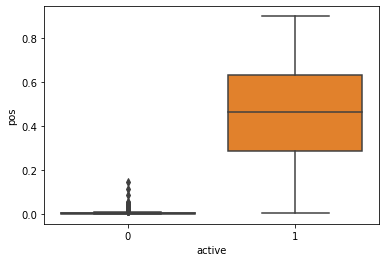
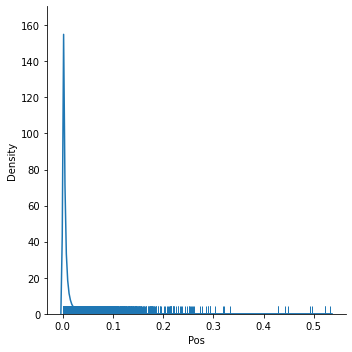
점수표의 전체 분포 구조를 파악할 때 분포표 플롯은 아주 근사한 방법입니다. 이를 토대로 전체 분자들 중에서 오직 한 줌에 속하는 이들만이 점수 >= 0.3 라인을 채운다는 정황을 직시하게 됩니다.
점수가 표기된 데이터프레임과 애초부터 SMILES 문자 정보를 구비한 앞쪽의 데이터프레임을 하나로 연동(Join)할 방법도 마련되어 있습니다. 이런 기능을 적용하면 상단 클래스의 화학 물체군에만 초점을 두게 될 시 확인 시간을 대폭 감축시켜 줍니다.
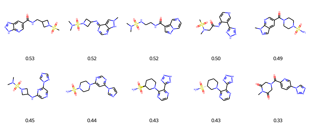
이러한 정보를 머금은 데이터프레임의 최상단 스코어를 보유한 히트작들에 화학적 구성의 가시화 결과를 결합 가능합니다.
| SMILES | Name | Val | Neg | Pos | Mol | |
|---|---|---|---|---|---|---|
| 46822 | CS(=O)(=O)N1CC(CNC(=O)c2cnc3[nH]nnc3c2)C1 | ZINC000428891788 | 0 | 0.467427 | 0.532573 |  |
| 76435 | CN(C)S(=O)(=O)N1CC(N=c2ncnc3[nH]n(C)cc2-3)C1 | ZINC000630384798 | 0 | 0.476829 | 0.523172 |  |
| 30397 | CN(C)S(=O)(=O)NCCNC(=O)c1cnn2ccncc12 | ZINC000353133002 | 0 | 0.478285 | 0.521715 |  |
| 95106 | CN(CC(=O)N=c1cc[nH]cc1-c1nn[nH]n1)S(C)(=O)=O | ZINC000736788034 | 0 | 0.503266 | 0.496734 |  |
| 54128 | Cn1ncc2cc(C(=O)N3CCN(S(N)(=O)=O)CC3)cnc21 | ZINC000530861476 | 0 | 0.506853 | 0.493147 |  |
위 화면의 결과를 확인하면 최상위 등급을 기록한 화합물 무리들의 구조가 상당 부분에서 동일한 패턴을 표출함을 확인할 수 있습니다. 시선을 돌려 상위권 이하 몇몇 분자 역시 마저 탐색해 보도록 합시다.
사실 수많은 화합물은 구조상 서로 꽤나 겹치는 유사 형태를 가진 관계로 우리가 필터링된 선발 단계에서 헛수고를 수반한 반복적인 잉여 처리만 거치게 할 가능성이 매우 농후합니다. 화합물 선발 스크리닝(screening)의 완성도를 높히면서 훨씬 효율적인 체계로 승급시키는 주요 해결 방안이 존재하는데, 분자 개체들을 특정 구획인 클러스터(cluster) 별로 분류시킨 뒤 그 중 오직 각 군집의 최고 랭크 데이터만을 채택하는 조치(Clustering)가 그 답안입니다. 이 방안 구현을 위해 널리 통용되는 유명 기법으로 RDKit-Butina 군집화(clustering) 시스템이 도입되었습니다. RDKit을 경유하면 놀라울만큼 간단한 소스코드만 거치고서도 순식간에 복잡한 클러스터 처리를 가뿐히 완성시킬 것입니다. Butina 로직에 적용될 오직 하나의 필요 지침 요소만 존재하는데 바로 파라미터 값인 임계점(cutoff) 점수입니다. 두 피실험의 Tanimoto 상관척도가 설정치 임계선을 초과할때만 같은 공동구역 클러스터 배정이 떨어집니다. 반대 현상으로 수치가 허들 밑을 기록할때 양측은 가차없이 갈라져 다른 군집 위치로 할당받게 됩니다.
클러스터링 처리가 시작되기도 전에 앞서 상위 점수판의 100위 랭크 안팎의 개체 대상으로만 범위를 압축하여 취합할 신규 데이터 프레임을 마련해 보겠습니다. 원래 콤보 정렬 과정에서 내림차순으로(sorted) 깔끔하게 세팅되었음을 참고하면 그야말로 “head” 코드 속성 하나만을 접목시키는 것을 통해 첫 순위부터 정확하게 하락하여 100항 행 부분까지만 포장할 수 있게 됩니다.
이어지는 진행으로 각각 분자 집단 별도의 식별 기준 코드가 기재될 새 컬럼(column) 영역을 이 데이터프레임 상에 창설하게 됩니다.
| SMILES | Name | Val | Neg | Pos | Mol | Cluster | |
|---|---|---|---|---|---|---|---|
| 46822 | CS(=O)(=O)N1CC(CNC(=O)c2cnc3[nH]nnc3c2)C1 | ZINC000428891788 | 0 | 0.467427 | 0.532573 | |
90 |
| 76435 | CN(C)S(=O)(=O)N1CC(N=c2ncnc3[nH]n(C)cc2-3)C1 | ZINC000630384798 | 0 | 0.476829 | 0.523172 | |
89 |
| 30397 | CN(C)S(=O)(=O)NCCNC(=O)c1cnn2ccncc12 | ZINC000353133002 | 0 | 0.478285 | 0.521715 | |
88 |
| 95106 | CN(CC(=O)N=c1cc[nH]cc1-c1nn[nH]n1)S(C)(=O)=O | ZINC000736788034 | 0 | 0.503266 | 0.496734 | |
87 |
| 54128 | Cn1ncc2cc(C(=O)N3CCN(S(N)(=O)=O)CC3)cnc21 | ZINC000530861476 | 0 | 0.506853 | 0.493147 | |
86 |
이제 우리 손에 들어온 이 다수의 클러스터 종류가 실제로 대관절 얼마나 독창적인 숫자 묶음을 배출했을지 알아보기 위함으로 “unique” 단축키 코드의 기능을 빌릴 수 있습니다.
90모든 과정 속에서 우리의 가장 우선적 목적은 결과 도출을 이끌어 낸 최고 명단 화합물 샘플을 확보, 구매 하는 데 있습니다. 이 마지막의 숙원 작업을 실현하려면 최종 획득 물품 화합물 리스트를 별도 보존할 csv 장부 기록으로의 편입이 무척이나 시급합니다. Pandas 명령어 기반의 “drop_duplicates” 모델을 개입시킬 경우 1개 구획의 맵 클러스터에서 최우수 분자 리스트 1항목만 분별 선정한 후 잔여 나머지는 삭제시킬 수 있습니다. 원리상 본 기능 구동 시 가장 높은 상단부의 기초 기록물부터 단계마다 갱신되며 똑같은 값이 재차 노출될 시 그 하단 목록 개체를 제거시켜나가는 법칙에서 기인하게 됨을 주시하여 주십시오.
(90, 7)