scRNA데이터 전처리하기

Taeyoon Kim

2023-09-22 11:57

시작하기 앞서¶

다음과 같은 몇가지 가정을 하고 시작하겠습니다.

가정1. 10x Genomics Single Cell Solution을 통해 얻은 서열 데이터를 사용
가정2. 리눅스(Ubuntu 22.04.3 LTS x86_64) OS를 사용하며 기본적인 shell 명령어를 앎
가정3. 패키지 매니저인 Anaconda에 대한 사용법을 알고 있음

터미널을 열고 원하는 폴더로 이동합니다. 저는 /home/fkt/Downloads에서 시작하도록 하겠습니다.

$pwd
/home/fkt/Downloads

가상환경 만들기¶

다음과 같이 사용가상환경을 만들어 사용합니다. 먼저 TutorialEnvironment.yml 파일을 다음 명령어로 다운받습니다.

해당 파일에는 RNA velocity 분석을 위한 velocyto 도구의 dependancy 정보가 들어 있습니다.

wget https://cf.10xgenomics.com/supp/cell-exp/neutrophils/TutorialEnvironment.yml

다음 명령어로 가상환경을 만들어 줍니다.

conda env create --file TutorialEnvironment.yml

만들어진 가상환경을 활성화 시킵니다.

conda activate tutorial

다운로드 받은 yml파일은 삭제해줍니다.

rm TutorialEnvironment.yml

Cell ranger 설치¶

10x Genomics Single Cell Solution을 통해 single cell RNA sequncing을 했다면 10x Genomics에서 Cell ranger라는 alignment 도구를 제공하고 있습니다. 속도는 좀 느려도 사용 용이성은 좋아서 저는 Cellranger를 추천합니다. 자세한 것은 공식사이트를 참고하시기 바랍니다.

시스템 요구사항¶

Cellranger는 리눅스 시스템에서 작동하며 다음의 최소 사양을 요구합니다:

8-core Intel or AMD processor (16 cores recommended).
64GB RAM (128GB recommended).
1TB free disk space.
64-bit CentOS/RedHat 7.0 or Ubuntu 14.04 - See the 10x Genomics OS Support page for details.

터미널에 다음 명령어를 입력해 cell ranger 7.2버전을 다운로드 합니다.

현재 기준으로 7.2 버전이 최신입니다.

wget -O cellranger-7.2.0.tar.gz "https://cf.10xgenomics.com/releases/cell-exp/cellranger-7.2.0.tar.gz?Expires=1695129121&Key-Pair-Id=APKAI7S6A5RYOXBWRPDA&Signature=ZipqR8Pg4YvVDQ3MvAVuuiPwEOC5c39~Wj0WTAxfoJW6xtrxqIFgIDySFSFnsWcwDpmAovJGrHXU24Y9Cptt88OJSPdEupyFRXoGKJvVzRtDJChmuMbSpVCy-2N-QnMKwxNtd8Yt8Mdp2Vcq4wxx1hVC0Yx54c7U9o~RFXIVsIp48thKR6JnKhJmCAC5U4dFLa86~NcB4s5Ic4HATrQP2KyWexyYZWgmBEw13mlKYtlVRUil0zseoq0-CZyGmE8oB0iDBSUBAyIqo~XMVjv~lkMz4cRcyCbQKBRDr~U36FM2KnE3rhv-Rlp4KD-uXCReRnBsY6N6t-HxpS2YDpN3mQ__"

그리고 나서 다음 명령어로 압축을 풀어줍니다.

tar -xvf cellranger-7.2.0.tar.gz

cellranger-7.2.0 폴더로 이동하기

cd cellranger-7.2.0

정상적으로 되었다면 아래와 같은 폴더 구조를 볼 수 있습니다.

.
├── bin
├── builtwith.json
├── cellranger -> bin/cellranger
├── external
├── lib
├── LICENSE
├── mro
├── probe_sets -> external/tenx_feature_references/targeted_panels
├── sourceme.bash
├── sourceme.csh
└── THIRD-PARTY-LICENSES.cellranger.txt

5 directories, 6 files

이제 ./cellranger명령어를 입력하면 아래와 같이 cell ranger 실행이 가능합니다.

./cellranger
cellranger cellranger-7.2.0

Process 10x Genomics Gene Expression, Feature Barcode, and Immune Profiling data

Usage: cellranger <COMMAND>

Commands:
  count           Count gene expression and/or feature barcode reads from a single sample and GEM well
(중략)
  help            Print this message or the help of the given subcommand(s)

Options:
  -h, --help     Print help
  -V, --version  Print version

FASTQ 파일과 레퍼런스 데이터 준비¶

10x Genomics사에서는 학습을 위한 데이터를 제공하고 있습니다. 이미 많은 예제에서 Human 1k PBMC를 다루고 있으므로 저는 Mouse 1k neuron으로 진행해보겠습니다. Human 1k PBMC은 직접해보시기 바랍니다.

Human PBMC 1k 데이터 다운로드¶

터미널에 다음과 같이 입력합니다.

mkdir data && cd data
#  Human PBMC 1k = 5.17GB
wget https://cf.10xgenomics.com/samples/cell-exp/3.0.0/pbmc_1k_v3/pbmc_1k_v3_fastqs.tar
tar -xvf pbmc_1k_v3_fastqs.tar
# Human reference (GRCh38) = 11GB
wget https://cf.10xgenomics.com/supp/cell-exp/refdata-gex-GRCh38-2020-A.tar.gz
tar -zxvf refdata-gex-GRCh38-2020-A.tar.gz

Mouse 1k neuron 데이터 다운로드¶

터미널에 다음과 같이 입력합니다.

# Mouse neron 1k data = 7GB
wget http://cf.10xgenomics.com/samples/cell-exp/3.0.0/neuron_1k_v3/neuron_1k_v3_fastqs.tar
tar -xvf neuron_1k_v3_fastqs.tar
# Mouse reference = 9.7GB
wget https://cf.10xgenomics.com/supp/cell-exp/refdata-gex-mm10-2020-A.tar.gz
tar -zxvf refdata-gex-mm10-2020-A.tar.gz

다운로드된 파일 확인¶

정상적으로 진행되었다면 아래와 같은 폴더와 52개의 파일을 확인할 수 있습니다.

$ tree .
.
├── neuron_1k_v3_fastqs
│   ├── neuron_1k_v3_S1_L001_I1_001.fastq.gz
│   ├── neuron_1k_v3_S1_L001_R1_001.fastq.gz
│   ├── neuron_1k_v3_S1_L001_R2_001.fastq.gz
│   ├── neuron_1k_v3_S1_L002_I1_001.fastq.gz
│   ├── neuron_1k_v3_S1_L002_R1_001.fastq.gz
│   └── neuron_1k_v3_S1_L002_R2_001.fastq.gz
├── pbmc_1k_v3_fastqs
│   ├── pbmc_1k_v3_S1_L001_I1_001.fastq.gz
│   ├── pbmc_1k_v3_S1_L001_R1_001.fastq.gz
│   ├── pbmc_1k_v3_S1_L001_R2_001.fastq.gz
│   ├── pbmc_1k_v3_S1_L002_I1_001.fastq.gz
│   ├── pbmc_1k_v3_S1_L002_R1_001.fastq.gz
│   └── pbmc_1k_v3_S1_L002_R2_001.fastq.gz
├── refdata-gex-GRCh38-2020-A
│   ├── fasta
│   ├── genes
│   │   └── genes.gtf
│   ├── pickle
│   ├── reference.json
│   └── star
└── refdata-gex-mm10-2020-A
    ├── fasta
    ├── genes
    │   └── genes.gtf
    ├── pickle
    ├── reference.json
    └── star

12 directories, 52 files

Cell ranger 사용하기¶

데이터가 준비되었으니 Cell ranger를 사용해 count matrix를 만들어 보겠습니다. 먼저 상위 디렉토리인 cellranger-7.2.0으로 이동합니다.

cd ..

다음과 같이 cellranger count 명령어를 사용하면 count matrix데이터를 얻을 수 있습니다.

./cellranger count --id=run_count_mNeuron1k \
--fastqs=data/neuron_1k_v3_fastqs  \
--sample=neuron_1k_v3  \
--transcriptome=data/refdata-gex-mm10-2020-A

--id는 생성되는 폴더명이며 --fastqs는 다운로드한 fastq파일의 위치입니다. --sample은 fastq 파일명의 접두사(prefix)를 의미하고 --transcriptome은 레퍼런스데이터의 위치입니다.

시간이 좀 지나면 다음과 같은 출력을 볼 수 있습니다.

Running preflight checks (please wait)...
Checking sample info...
Checking FASTQ folder...
Checking reference...
(후략)

정상적으로 작업이 완료된다면 아래처럼 outs이라는 폴더가 생성됩니다. 여기에는 count matrix뿐만 아니라 여러가지 분석 결과도 포함되어 있어 복잡해보입니다. 그러나 저희가 필요 한 것은 filtered_feature_bc_matrix 폴더 안에 다들어 있습니다.

outs
├── analysis
├── cloupe.cloupe
├── filtered_feature_bc_matrix
├── filtered_feature_bc_matrix.h5
├── metrics_summary.csv
├── molecule_info.h5
├── possorted_genome_bam.bam
├── possorted_genome_bam.bam.bai
├── raw_feature_bc_matrix
├── raw_feature_bc_matrix.h5
└── web_summary.html

RNA velocity 분석을 위한 작업¶

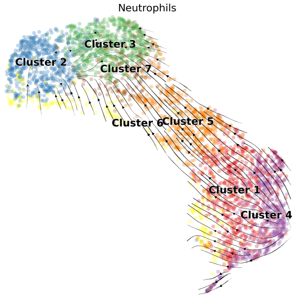
RNA velocity이란? 스플라이싱된 RNA와 아직 스플라이싱되지 않은 RNA를 구분해 세포의 상태를 예측하는 기법으로 scRNA 데이터에서 클러스터간에 분화 과정에 대한 단서를 얻을 수 있습니다. 예를 들어 아래 그림에서 보면 cluster4에서 cluster2로의 방향성을 확인 할 수 있습니다.

안타깝게도 Cell ranger를 통해 얻은 count matrix로는 RNA velocity 분석을 할 수 없습니다. 추가적으로 velocyto이라는 도구를 사용해 unspliced , spliced 데이터가 포함된 loom파일을 만들어야 합니다. 아래 명령어를 사용하면 간단하게 얻을 수 있습니다.

velocyto run10x run_count_mNeuron1k/ data/refdata-gex-mm10-2020-A/genes/genes.gtf

실행이 완료되는 시간은 생각보다 오래 걸립니다.

2023-09-19 10:01:22,756 - DEBUG - Using logic: Default
2023-09-19 10:01:22,757 - DEBUG - Example of barcode: AAACGAATCAAAGCCT and cell_id: run_count_mNeuron1k:AAACGAATCAAAGCCT-1
(중략)
2023-09-19 10:27:23,985 - DEBUG - 1991314 reads were skipped because no apropiate cell or umi barcode was found
2023-09-19 10:27:23,985 - DEBUG - Counting done!
2023-09-19 10:27:23,988 - DEBUG - Collecting row attributes
2023-09-19 10:27:24,014 - DEBUG - Generating data table
2023-09-19 10:27:24,056 - DEBUG - Writing loom file
2023-09-19 10:27:25,286 - DEBUG - Terminated Succesfully!

완료가 되면 run_count_mNeuron1k폴더안에 velocyto라는 새로운 폴더가 생기고 run_count_mNeuron1k.loom 파일이 생성됩니다.

Count matrix 데이터 읽기¶

이제 힘든 데이터 준비 과정이 모두 끝났습니다. 데이터 분석을 시작해보죠. scRNA-seq 분야는 아직 초기이고 새로운 도구들이 계속 쏟아지고 있습니다. 나중은 어떻게 될지 모르겠지만 지금 시점에서는 R에 익숙하다면 Seurat, Python에 익숙하다면 Scanpy를 추천합니다.

참고로 속도적인 측면과 ML을 접목하기에는 Scanpy가 더 강점을 가지고 있습니다.

Scanpy 사용하기¶

다음 코드를 통해 count matrix를 scanpy로 불러 올 수 있습니다.

In [1]:

# conda install pandas scanpy
import scanpy as sc

# Cell ranger 결과 파일이 들어있는 경로
file_path = "../input/run_count_mNeuron1k/outs/filtered_feature_bc_matrix"

# read_10x_mtx 함수를 사용
adata = sc.read_10x_mtx(file_path, var_names="gene_symbols", cache=True)
adata

Out[1]:

AnnData object with n_obs × n_vars = 1311 × 32285
    var: 'gene_ids', 'feature_types'

scVelo를 사용해 RNA velocity분석을 한다면 아래의 추가적인 코드가 필요합니다.

In [2]:

# conda install -c bioconda scvelo
import scvelo as scv

# load loom files for spliced/unspliced matrices for each sample
loom = scv.read(f"{file_path}/run_count_mNeuron1k.loom", validate=False, cache=False)

# rename barcodes in order to merge:
barcodes = [bc.split(":")[1] for bc in loom.obs.index.tolist()]
barcodes = [bc[0 : len(bc) - 1] + "-1" for bc in barcodes]
loom.obs.index = barcodes

# make variable names unique
loom.var_names_make_unique()

# merge matrices into the original adata object
adata = scv.utils.merge(adata, loom)
adata

Out[2]:

AnnData object with n_obs × n_vars = 1311 × 32285
    obs: 'initial_size_unspliced', 'initial_size_spliced', 'initial_size'
    var: 'gene_ids', 'feature_types', 'Accession', 'Chromosome', 'End', 'Start', 'Strand'
    layers: 'matrix', 'ambiguous', 'spliced', 'unspliced'

In [3]:

scv.pl.proportions(adata)

No description has been provided for this image

scanpy는 *.h5ad 포멧을 사용해 count matrix를 저장합니다. 아래 코드를 사용하면 단일 파일로 모든 것을 저장할 수 있습니다.

In [ ]:

adata.write("../output/mNeuron1k.h5ad", compression="gzip")

Seurat 사용하기¶

R에 좀 더 익숙하시다면 Seurat을 사용하세요. 저는 파이썬 문법을 더 좋아하지만 솔직히 분석 도구의 완성도 측면에서는 Seurat이 더 나은 것 같습니다. 아래 코드는 jupyter notebook에서 R코드를 사용하기 위해 필요한 것으로 rStudio를 사용하신다면 %%R이 포함된 셀의 코드만 사용하시면 됩니다.

In [4]:

import logging
import rpy2.rinterface_lib.callbacks as rcb

# import rpy2.robjects as ro

rcb.logger.setLevel(logging.ERROR)
%load_ext rpy2.ipython

필요한 Seurat 라이브러리를 불러옵니다.

In [5]:

%%R
library(dplyr)
library(Seurat)

    WARNING: The R package "reticulate" only fixed recently
    an issue that caused a segfault when used with rpy2:
    https://github.com/rstudio/reticulate/pull/1188
    Make sure that you use a version of that package that includes
    the fix.

아래의 코드를 사용하면 count matrix를 Seurat object로 만들 수 있습니다.

In [6]:

%%R
# Load dataset
neuron.data <- Read10X(data.dir = "../input/run_count_mNeuron1k/outs/filtered_feature_bc_matrix")
# Initialize the Seurat object.
obj <- CreateSeuratObject(counts = neuron.data)
obj

An object of class Seurat 
32285 features across 1311 samples within 1 assay 
Active assay: RNA (32285 features, 0 variable features)

Seurat object를 파일로 저장하는 방법에도 여러가지가 있지만 R에서 많이 사용되는 *.rds를 사용하는 코드는 아래와 같습니다.

In [8]:

%%R
saveRDS(obj, file = "../output/mNeuron1k.rds")

마치며¶

이것으로 scRNA seq 데이터의 전처리 과정을 알아봤습니다. 여기 적힌 방법 외에도 더 효율적이고 나은 방법도 있고 앞으로도 더 생겨날 것입니다. 그러나 저도 배우는 입장에서 다른 분들에게 도움이 되고자 정리를 해봤습니다. 실제 실험을 통해 얻은 데이터를 분석하는데 도움이 되길 바랍니다.