파이썬으로 PK 분석하기

0. Pharmacokinetics(PK) 분석

ELISA를 이용하여 혈액에서 시험 약물의 약물학적 동태(Pharmacokinetics)를 평가한 데이터를 분석해보도록 하겠습니다. Pharmacokinetics(이하, PK)는 간단히 말하면 특정 약물에 대해서 몸이 어떻게 반응하는지를 보는 것입니다.

Pharmacokinetics은 약물의 흡수, 분포, 대사, 배설과정을 동역학적 관점에서 해석하고 예측하고자 하는 것이다. -- 위키백과

PK 분석을 통해서 약물의 반감기를 분석하고 약물 주입방식에 따른 차이를 살펴보도록 하겠습니다.

0.1. 실험 디자인

실험 쥐에 약물 X를 아래의 두가지 주입방식으로 실험합니다. 정확도를 위해 3번 반복하여 값을 측정하였습니다.

  • IV(intravenous injection): 정맥주사
  • SC(subcutaneous injection): 피하주사

주입후 72시간동안 실험 쥐의 혈액을 채취해 남아있는 약물 X의 양을 구합니다.

1. 데이터 불러오기

필요한 라이브러리를 불러옵니다.

In [1]:
# load modules
%matplotlib inline
import matplotlib.pyplot as plt
import pandas as pd

실험 결과를 정리한 CSV파일을 pd.read_csv()를 이용해 읽어옵니다.

In [2]:
# read csv file to analysis
df = pd.read_csv("./data/20180108_PK.csv")
num = df._get_numeric_data()  # 음수 값을 0으로
num[num < 0] = 0
df.sample(5)
Out[2]:
Inject Time(h) Sample Wells Value Result R
8 IV 8 8 C3 1.299 1.644 R
17 IV 48 20 C5 0.455 0.477 NaN
32 SC 8 35 F7 0.000 0.000 R
30 SC 8 33 D7 0.125 0.019 R
36 SC 24 39 D8 0.209 0.136 NaN

2. 데이터 전처리

Injection 방법에 의한 차이와 샘플을 채취한 시간, 실험용 쥐의 번호등을 확인 할 수 있습니다. 데이터 전처리 과정에서 필요없는 행을 삭제하고 반복측정한 값의 평균값과 표준편차를 계산하겠습니다.

In [3]:
# 필요없는 행 삭제
df = df.drop(["Sample", "Wells", "Value", "R"], axis=1)

# Inject 종류에 따라서 데이터 분리
df_IV = df[df["Inject"] == "IV"]
df_SC = df[df["Inject"] == "SC"]
df_IV.head()
Out[3]:
Inject Time(h) Result
0 IV 0 1.637
1 IV 0 1.853
2 IV 0 1.779
3 IV 4 1.591
4 IV 4 1.234

groupby()기능을 사용해 시간별로 그룹핑 합니다. 그런다음 평균값과 표준편차를 구합니다.

In [4]:
# 평균값
mean_IV = df_IV.groupby("Time(h)").mean()
mean_SC = df_SC.groupby("Time(h)").mean()
# 표준편차
std_IV = df_IV.groupby("Time(h)").std()
std_SC = df_SC.groupby("Time(h)").std()
mean_IV  # IV 테이블을 확인합니다.
Out[4]:
Result
Time(h)
0 1.756333
4 1.231333
8 1.655333
16 1.297000
32 1.092333
48 0.505667
64 0.102333
72 0.033333

데이터가 잘 정돈 된것을 확인했으니, 다음으로 시각화를 합니다.

2. 시각화하기

2.1. 간단한 선그래프

선그래프로 전체적인 모양을 확인해 봅니다.

In [5]:
plt.plot(mean_IV["Result"], "o-")  # IV 값
plt.plot(mean_SC["Result"], "o--")  # SC 값
Out[5]:
[<matplotlib.lines.Line2D at 0x7f6d0d8bc208>]
No description has been provided for this image

2.2. 선그래프에 에러바 추가하기

위의 그래프에서는 IV injection의 두번째 값이 좀 낮은 것 같은데, 표준편차가 표시되어 있지 않아 실제값 자체가 낮은 것인지 실험상의 편차인지 명확하지 않습니다. plt.errorbar()를 이용해서 에러바를 표시해 알아 보도록 하죠.

In [6]:
fig, ax = plt.subplots()
fig_name = "PK_analysis"
ax.set(title=fig_name, xlabel="Time(h)", ylabel="Activity(IU/ml)")
ax.errorbar(
    x=mean_IV.index.values,
    y=mean_IV["Result"],
    yerr=std_IV["Result"],
    fmt="o-",
    capsize=3,
    label="IV",
)
ax.errorbar(
    x=mean_SC.index.values,
    y=mean_SC["Result"],
    yerr=std_SC["Result"],
    fmt="o-",
    capsize=3,
    label="SC",
)
plt.legend()  # 범례 표시
ax.spines["right"].set_visible(False)  # 프레임 숨기기
ax.spines["top"].set_visible(False)
# plt.savefig(fig_name + '.png', dpi = 600 ) # 저장하기
No description has been provided for this image

IV injection의 두번째 값의 표준편차가 큰것을 확인할 수 있습니다. 따라서 실험상의 편차로 인해 나타난 현상이라고 볼 수 있겠습니다.

3. 반감기 계산

Pharmacokinetics 실험의 목적이라고 할 수 있는 약물의 반감기를 계산해 보도록 하겠습니다. 계산을 위해선 실험 데이터에 Curve fitting을 수행해야 합니다. 파이썬에서는 scipy.optimize.curve_fit() 을 사용하도록 하겠습니다.

In [7]:
# 필요한 라이브러리를 불러옵니다.
from scipy.optimize import curve_fit
import numpy as np
import warnings  # 경고를 무시합니다.

warnings.filterwarnings("ignore")

전체적인 PK 데이터의 모양을 보면 가장 간단한 one-compartment model를 사용하면 될 것 같습니다. 먼저 지수(exponential) 함수를 정의해 Curve fitting을 합니다.

In [8]:
def exponential(x, D, k):
    return D * np.exp(-k * x)

3.1. IV 주입 반감기

계산을 위해서는 IV 데이터를 numpy.array()로 변경해야 합니다.

Curve fitting

실험데이터를 가장 가깝게 모든데이터를 지나는 선을 그려봅니다.

In [18]:
x = np.array(mean_IV.index.values)
y = np.array(mean_IV["Result"])
# curve fitting 하기
popt, pcov = curve_fit(exponential, x, y)

ss_res = np.sum((y - exponential(x, *popt)) ** 2)  # residual sum of squares
ss_tot = np.sum((y - np.mean(y)) ** 2)  # total sum of squares
r2 = 1 - (ss_res / ss_tot)  # r-squared
print("R-squared is {:.3f}%.".format(r2 * 100))

# 시각화
xx = np.linspace(0, 80, 1000)
yy = exponential(xx, *popt)
plt.plot(x, y, "o")
plt.plot(xx, yy)
R-squared is 86.839%.
Out[18]:
[<matplotlib.lines.Line2D at 0x7f6cb825be10>]
No description has been provided for this image

두번째 포인트 값이 역시나 말썽입니다. 전체적인 R2값도 낮습니다. 몇개의 값을 제외하고 다시 해보겠습니다.

In [19]:
# 2번째, 4번째 데이터를 제외
selection = np.array([0, 2, 3, 5, 6, 7])
x = x[selection]
y = y[selection]
# curve fitting 하기
popt, pcov = curve_fit(exponential, x, y)

ss_res = np.sum((y - exponential(x, *popt)) ** 2)  # residual sum of squares
ss_tot = np.sum((y - np.mean(y)) ** 2)  # total sum of squares
r2 = 1 - (ss_res / ss_tot)  # r-squared
print("R-squared is {:.3f}%.".format(r2 * 100))

# 시각화
xx = np.linspace(0, 80, 1000)
yy = exponential(xx, *popt)
plt.plot(x, y, "o")
plt.plot(xx, yy)
R-squared is 95.712%.
Out[19]:
[<matplotlib.lines.Line2D at 0x7f6cb825bc18>]
No description has been provided for this image

아까보다는 좀 더 잘맞는 것 같습니다. 일단은 반감기를 구해보도록 하죠.

반감기 계산

반감기는 주입한 약물의 양이 1/2로 감소하는 데 소요되는 시간입니다. 반감기를 구하는 공식이 따로 있기는 합니다만, 여기서는 Curve fiiting에 사용한 함수의 역함수를 정의해서 주입한 약물양의 절반이 되는 시간을 구해보겠습니다.

In [20]:
half_y = exponential(0, *popt) / 2  # 주입한 약물량을 2로 나누어 줍니다


# 계산을 위한 역함수를 정의합니다.
def rev_log(y, D, k):
    """for halflife calculate"""
    return (np.log(y) - np.log(D)) / -k


half_life = rev_log(half_y, *popt)
print("반감기는 {:.2f} 시간 입니다.".format(half_life))
# print(0.693/popt[1]) # Equation 에 의해 계산되는 값
반감기는 22.53 시간 입니다.

3.2. SC 주입 반감기

SC 경우는 처음에는 약물이 흡수되는 시간이 있습니다. 그래서 처음 3개의 결과는 제외하고 반감기를 구해보겠습니다.

Curve fitting

In [21]:
x = np.array(mean_SC.index.values)
y = np.array(mean_SC["Result"])
x = x[3:]
y = y[3:]

# curve fitting 하기
popt, pcov = curve_fit(exponential, x, y)

ss_res = np.sum((y - exponential(x, *popt)) ** 2)  # residual sum of squares
ss_tot = np.sum((y - np.mean(y)) ** 2)  # total sum of squares
r2 = 1 - (ss_res / ss_tot)  # r-squared
print("R-squared is {:.3f}%.".format(r2 * 100))

# 시각화
xx = np.linspace(16, 80, 1000)
yy = exponential(xx, *popt)
plt.plot(x, y, "o")
plt.plot(xx, yy)
R-squared is 99.541%.
Out[21]:
[<matplotlib.lines.Line2D at 0x7f6cb7d89cf8>]
No description has been provided for this image

반감기 계산

In [22]:
half_y = exponential(16, *popt) / 2  # 주입한 약물량을 2로 나누어 줍니다


# 계산을 위한 역함수를 정의합니다.
def rev_log(y, D, k):
    """for halflife calculate"""
    return (np.log(y) - np.log(D)) / -k


half_life = rev_log(half_y, *popt)
print("반감기는 {:.2f} 시간 입니다.".format(half_life))
반감기는 19.93 시간 입니다.

4. Bioavailability(BA) 계산

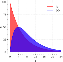
약물의 흡수는 생체 이용률(bioavailability)로 나타내는데, 경구로 투여된 약물이 전신순환계에 들어가 생체에 이용되는 비율을 말하며, 투여 후 혈중 약물 농도의 총 면적, 즉 AUC(Area Under the Concentration- time Curve)가 생체 이용률의 지표로 흔히 쓰이고 있다. -- Kyung Soo Kim, et al. Drug Effect and Generic Substitution

4.1. The absolute bioavailability

정맥투여에 대한 상대적인 흡수율을 나타내며, %로 표시하기에 절대적 생체 이용률이라고 한다. 약 물을 정맥에 투여할 때에는 곧 바로 전신순환에 도달되기 때문에 전신약물 흡수 즉 생체 이용률은 100%으로 생각한다. -- Kyung Soo Kim, et al. Drug Effect and Generic Substitution

아래의 공식은 절대적 생체 이용률(BA)를 구하는 방법입니다.

  • po = Oral route; 경구투여
  • iv = Intravenous injection; 정맥주사
  • D = Dose; 투여량

이번 예시에서는 경구투여대신 SC(피하주사) 데이터를 사용해 절대 생체 이용률을 구해 보겠습니다. 파이썬에서는 sklearn.metrics() 기능을 사용해 손쉽게 그래프의 AUC를 구할 수 있습니다. 각각의 AUC를 구해서 상대적 비교를 하면 BA를 계산할 수 있습니다.

In [24]:
from sklearn import metrics  # 필요한 라이브러리 불러오기

x1 = np.array(mean_IV.index.values)
y1 = np.array(mean_IV["Result"])
x2 = np.array(mean_SC.index.values)
y2 = np.array(mean_SC["Result"])

# 각각의 AUC를 구합니다.
IV_auc = metrics.auc(x1, y1)
SC_auc = metrics.auc(x2, y2)
IV_conc = 100
SC_conc = 50
# 수식에 맞춰 BA를 계산합니다.
BA = (SC_auc * IV_conc) / (IV_auc * SC_conc)

print("Bioavailability of SC injection is {:.2f}%.".format(BA * 100))
Bioavailability of SC injection is 12.14%.

5. 마치며

이번 포스트에서는 파이썬을 이용해 간단한 PK 분석을 해보았습니다. 저도 이쪽의 전문가가 아니라 직접 찾아보며 계산했습니다. 틀린 부분이 있다면 이해해주시기 바랍니다. 약물의 반감기와 BA는 다양한 PK 변수중에 극히 일부이지만, 이러한 변수를 구하는 방법을 안다면 다른 변수들도 쉽게 계산할 수 있으실 것입니다.

ggpubr로 논문급 도표그리기

0. ggpubr

모든 내용은 공식문서에서 간추린 것입니다. 자세한것은 공식문서를 읽어주세요.

ggpubr은 ggplot2에 기반한 R 패키지입니다. 연구자들이 쉽게 높은 질의 도표를 그리는 것을 목표로 하고 있는 시각화 패키지죠. 주요 특징은 다음과 같습니다:

  • ggplot2 패키지를 기반으로해서 좀 더 명확한 문법으로 보다 쉽게 사용할 수 있습니다.
  • R 언어를 잘 모르더라도 높은 질의 도표를 만들수 있습니다.
  • 자동으로 p-values 나 통계적 유의성을 표시할 할 수 있습니다.
  • 여러 도표를 한 페이지에 배열 할 수 있는 기능을 가지고 있습니다.
  • 레이블이나 색상을 쉽게 변경할 수 있습니다.

먼저 ggpubr 로 시각화를 하는 간단한 방법을 살펴보고, 이후에 다양한 예시 도표를 보여드리겠습니다.

1. ggpubr 설치하기:

CRAN 을 통한 설치법은 아래와 같습니다.

install.packages("ggpubr")

2. ggpubr 불러오기:

library("ggpubr")

3. ggpubr로 도표 그리기

간단한 예시를 들어 시각화 방법을 살펴보겠습니다.

  1. 대이터 불러와서 전처리하기
  2. 시각화하고 설정하기

3.1. 데이터 불러오기

In [2]:
# 필요한  패키지 불러오기
library("dplyr") 
library("ggpubr")
options(warn=-1) # 경고메세지 무시하기

data("ToothGrowth") # 예제 데이터 불러오기
head(ToothGrowth,4) # 데이터 테이블 확인
len supp dose
4.2 VC 0.5
11.5 VC 0.5
7.3 VC 0.5
5.8 VC 0.5

3.2. 시각화 설정하기

In [3]:
ggline(ToothGrowth, x = "dose", y = "len", add = "mean_se", # 각각의 축설정 
      color = "supp", palette = "npg")+  # 색상 설정하기
      stat_compare_means(aes(group = supp), label = "p.signif", label.y = c(16, 25, 29)) + # 통계적 유의성 표시
      labs(list(x = 'Dose', y = 'Length', fill = 'Supp')) # 레이블 변경
No description has been provided for this image

3.3. 한페이지에 여러 도표 넣기

여러 도표를 한페이지에 넣는 기능은 ggarrange()입니다. cowplot plot_grid()함수에 기반하고 있죠. 그래서 사용법도 동일합니다. 아래의 예시 코드를 확인하세요.

ggarrange(a, b, c ,  
          labels = c("A", "B", "C"),
          ncol = 2, nrow = 2)

4. 다양한 ggpubr 예시

아래에는 많이 사용되는 도표의 예시를 제공하고 있습니다. 필요한 것이 있는지 살펴보세요.

4.1. 분포(Distribution) 시각화

In [4]:
# 예제 데이터 만들기
set.seed(1234)
wdata = data.frame(
   sex = factor(rep(c("F", "M"), each=200)),
   weight = c(rnorm(200, 55), rnorm(200, 58)))
head(wdata, 4)
sex weight
F 53.79293
F 55.27743
F 56.08444
F 52.65430
In [5]:
a1 <- ggdensity(wdata, x = "weight",
   add = "mean", rug = TRUE, # Density plot with mean lines and marginal rug
   color = "sex", fill = "sex",  # Change outline and fill colors by groups ("sex")
   palette = c("#00AFBB", "#E7B800")) # Use custom palette

a2 <- gghistogram(wdata, x = "weight",
   add = "mean", rug = TRUE,
   color = "sex", fill = "sex",
   palette = c("#00AFBB", "#E7B800"))

a3 <- ggdensity(wdata, x = "weight",
   add = "mean", rug = TRUE,
   fill = "lightgray")

# Combine histogram and density plots
a4 <-  gghistogram(wdata, x = "weight",
   add = "mean", rug = FALSE,
   fill = "sex", palette = c("#00AFBB", "#E7B800"),
   add_density = TRUE)

# 한페이지에 넣기
ggarrange(a1, a2, a3 , a4,
          labels = c("A", "B", "C", "D"),
          ncol = 2, nrow = 2)
No description has been provided for this image

4.2. 박스 그래프(Box plots), 바이올린(violin plots) 그래프

In [6]:
# Load data
data("ToothGrowth")
df <- ToothGrowth
head(df, 4)
len supp dose
4.2 VC 0.5
11.5 VC 0.5
7.3 VC 0.5
5.8 VC 0.5
In [7]:
# Box plots with jittered points
p1 <- ggboxplot(df, x = "dose", y = "len",
        color = "dose", palette =c("#00AFBB", "#E7B800", "#FC4E07"),
        add = "jitter", shape = "dose")

# Add p-values comparing groups
my_comparisons <- list( c("0.5", "1"), c("1", "2"), c("0.5", "2") )
p2 <- p1 + stat_compare_means(comparisons = my_comparisons)+ # Add pairwise comparisons p-value
        stat_compare_means(label.y = 50)                   # Add global p-value

# Violin plots with box plots inside
p3 <- ggviolin(df, x = "dose", y = "len", fill = "dose",
         palette = c("#00AFBB", "#E7B800", "#FC4E07"),
         add = "boxplot", add.params = list(fill = "white"))+
         stat_compare_means(comparisons = my_comparisons, label = "p.signif")+ # Add significance levels
         stat_compare_means(label.y = 50)        # Add global the p-value 

ggarrange(p1, p2, p3,
          labels = c("A", "B", "C"),
          ncol = 2, nrow = 2)
No description has been provided for this image

4.3. 막대 그래프(Bar plots)

4.3.1 간단한 막대 그래프

In [8]:
# example Data
df <- data.frame(dose=c("D0.5", "D1", "D2"),
   len=c(4.2, 10, 29.5))
df2 <- data.frame(supp=rep(c("VC", "OJ"), each=3),
   dose=rep(c("D0.5", "D1", "D2"),2),
   len=c(6.8, 15, 33, 4.2, 10, 29.5))
df3 <- ToothGrowth

# Change position: Interleaved (dodged) bar plot
p1 <- ggbarplot(df2, "dose", "len",
        fill = "supp", color = "supp", palette = "Paired",
        position = position_dodge(0.8))

# Change fill and outline color add labels inside bars
p2 <- ggbarplot(df, "dose", "len",
        fill = "dose", color = "dose",
        palette = c("#00AFBB", "#E7B800", "#FC4E07"),
        label = TRUE, lab.pos = "in", lab.col = "white")

# Add jitter points and errors (mean_se)
p3 <- ggbarplot(df3, x = "dose", y = "len",
        add = c("mean_se", "jitter"))

# Multiple groups with error bars and jitter point
p4 <- ggbarplot(df3, x = "dose", y = "len", color = "supp",
         add = "mean_se", palette = c("#00AFBB", "#E7B800"),
         position = position_dodge(0.8))

ggarrange(p1, p2, p3, p4,
          labels = c("A", "B", "C", "D"),
          ncol = 2, nrow = 2)
No description has been provided for this image

4.3.2 정돈된(Ordered) 바 그래프

cyl에 따라서 그룹화하고, 전체적으로 정렬한 그래프(A)와 그룹별로 정렬한 그래프(B)의 시각화입니다.

In [9]:
# 샘플 데이터 불러오기
data("mtcars")
dfm <- mtcars
dfm$cyl <- as.factor(dfm$cyl) # Convert the cyl variable to a factor
dfm$name <- rownames(dfm) # Add the name colums
head(dfm[, c("name", "wt", "mpg", "cyl")]) # 데이터 살펴보기
name wt mpg cyl
Mazda RX4 Mazda RX4 2.620 21.0 6
Mazda RX4 Wag Mazda RX4 Wag 2.875 21.0 6
Datsun 710 Datsun 710 2.320 22.8 4
Hornet 4 Drive Hornet 4 Drive 3.215 21.4 6
Hornet Sportabout Hornet Sportabout 3.440 18.7 8
Valiant Valiant 3.460 18.1 6
In [10]:
a1 <- ggbarplot(dfm, x = "name", y = "mpg",
          fill = "cyl",               # change fill color by cyl
          color = "white",            # Set bar border colors to white
          palette = "jco",            # jco journal color palett. see ?ggpar
          sort.val = "desc",          # Sort the value in dscending order
          sort.by.groups = FALSE,     # Don't sort inside each group
          x.text.angle = 90)           # Rotate vertically x axis texts

a2 <- ggbarplot(dfm, x = "name", y = "mpg",
          fill = "cyl",               # change fill color by cyl
          color = "white",            # Set bar border colors to white
          palette = "jco",            # jco journal color palett. see ?ggpar
          sort.val = "asc",           # Sort the value in dscending order
          sort.by.groups = TRUE,      # Sort inside each group
          x.text.angle = 90)           # Rotate vertically x axis texts

ggarrange(a1, a2,
          labels = c("A", "B"),
          ncol = 1, nrow = 2)
No description has been provided for this image

4.3.3. 편차(Deviation) 그래프

편차(deviation) 그래프는 각각의 값들이 평균값 대비 얼마나 차이가 나는지를 시각화 합니다. 여기서는 연비 평균값에 비교해서 각 차량의 편차가 얼마인지 계산해(Z-score) 도표를 그려보겠습니다.

In [11]:
# Calculate the z-score of the mpg data
dfm$mpg_z <- (dfm$mpg -mean(dfm$mpg))/sd(dfm$mpg)
dfm$mpg_grp <- factor(ifelse(dfm$mpg_z < 0, "low", "high"), 
                     levels = c("low", "high"))
# Inspect the data
head(dfm[, c("name", "wt", "mpg", "mpg_z", "mpg_grp", "cyl")])
name wt mpg mpg_z mpg_grp cyl
Mazda RX4 Mazda RX4 2.620 21.0 0.1508848 high 6
Mazda RX4 Wag Mazda RX4 Wag 2.875 21.0 0.1508848 high 6
Datsun 710 Datsun 710 2.320 22.8 0.4495434 high 4
Hornet 4 Drive Hornet 4 Drive 3.215 21.4 0.2172534 high 6
Hornet Sportabout Hornet Sportabout 3.440 18.7 -0.2307345 low 8
Valiant Valiant 3.460 18.1 -0.3302874 low 6
In [12]:
# Create an ordered bar plot, colored according to the level of mpg:
ggbarplot(dfm, x = "name", y = "mpg_z",
          fill = "mpg_grp",           # change fill color by mpg_level
          color = "white",            # Set bar border colors to white
          palette = "jco",            # jco journal color palett. see ?ggpar
          sort.val = "desc",          # Sort the value in descending order
          sort.by.groups = FALSE,     # Don't sort inside each group
          x.text.angle = 90,          # Rotate vertically x axis texts
          ylab = "MPG z-score",
          legend.title = "MPG Group",
          rotate = TRUE,
          ggtheme = theme_minimal())
No description has been provided for this image

4.4 점 그래프(Dot plot)

4.4.1 막대사탕(Lollipop) plot

막대사탕 그래프는 많은 양의 데이터를 시각화하는데 적합합니다. 아래 예시에서는 cyl 그룹에 맞춰서 색상을 구분하였습니다.

In [13]:
ggdotchart(dfm, x = "name", y = "mpg",
           color = "cyl",                                # Color by groups
           palette = c("#00AFBB", "#E7B800", "#FC4E07"), # Custom color palette
           sorting = "descending",                       # Sort value in descending order
           add = "segments",                             # Add segments from y = 0 to dots
           rotate = TRUE,                                # Rotate vertically
           group = "cyl",                                # Order by groups
           dot.size = 6,                                 # Large dot size
           label = round(dfm$mpg),                        # Add mpg values as dot labels
           font.label = list(color = "white", size = 9, 
           vjust = 0.5),               # Adjust label parameters
           ggtheme = theme_pubr())                        # ggplot2 theme
No description has been provided for this image

4.5. 도표에 설명(figure legend) 넣기

도표 밑에 설명을 넣는 방법입니다. 한줄단위로 내용을 끊어서 작성해야, 산출물에서 줄이 잘 맞게 할 수 있습니다. 아래의 예시 코드를 확인하세요.

ggparagraph(text, color = NULL, size = NULL, face = NULL, family = NULL,
  lineheight = NULL)
# S3 method for splitText
drawDetails(x, recording)
In [14]:
# Density plot
density.p <- ggdensity(iris, x = "Sepal.Length",
                      fill = "Species", palette = "jco")
# Text plot
text <- paste("Iris data set gives the measurements in cm",
             "of the variables sepal length and width",
             "and petal length and width, respectively,",
             "for 50 flowers from each of 3 species of iris.",
             "The species are Iris setosa, versicolor, and virginica.", sep = " ")
text.p <- ggparagraph(text, face = "italic", size = 12)

# Arrange the plots on the same page
ggarrange(density.p, text.p,
         ncol = 1, nrow = 2,
         heights = c(1, 0.3))
No description has been provided for this image

4.6. 선 그래프

In [15]:
# Data: ToothGrowth data set we'll be used.
df3 <- ToothGrowth
# Add error bars: mean_se
# (other values include: mean_sd, mean_ci, median_iqr, ....)
# Add labels
p1 <- ggline(df3, x = "dose", y = "len", add = "mean_se")
# Add jitter points and errors (mean_se)
p2 <- ggline(df3, x = "dose", y = "len",
 add = c("mean_se",'jitter'))
# Multiple groups with error bars
p3 <- ggline(df3, x = "dose", y = "len", color = "supp",
 add = "mean_se", palette = c("#00AFBB", "#FC4E07"))

ggarrange(p1, p2, p3,
          labels = c("A", "B", "C"),
          ncol = 2, nrow = 2)
No description has been provided for this image

4.7. 히스토그램과 산포도(Scatter Plot with Histograms)

히스토그램과 산포도를 하나의 도표에 합쳐서 그려보도록 하겠습니다.

In [16]:
# Grouped data
ggscatterhist(
 iris, x = "Sepal.Length", y = "Sepal.Width",
 color = "Species", size = 3, alpha = 0.6,
 palette = c("#00AFBB", "#E7B800", "#FC4E07"),
 margin.params = list(fill = "Species", color = "black", size = 0.2))
No description has been provided for this image

4.8. 상관분석(Correlation Coefficients)과 P-values 추가하기

산포도에 상관분석p-values를 추가하는 방법입니다.

In [17]:
# Load data
data("mtcars")
df <- mtcars
df$cyl <- as.factor(df$cyl)

# Scatter plot with correlation coefficient
sp <- ggscatter(df, x = "wt", y = "mpg",
   add = "reg.line",  # Add regressin line
   add.params = list(color = "blue", fill = "lightgray"), # Customize reg. line
   conf.int = TRUE) # Add confidence interval
# Add correlation coefficient
p1 <- sp + stat_cor(method = "pearson", label.x = 3, label.y = 30)
# Color by groups and facet
sp <- ggscatter(df, x = "wt", y = "mpg",
   color = "cyl", palette = "jco",
   add = "reg.line", conf.int = TRUE)
p2 <- sp + stat_cor(aes(color = cyl), label.x = 3)
# Scatter plot with ellipses and group mean points
p3 <- ggscatter(df, x = "wt", y = "mpg",
   color = "cyl", shape = "cyl",
   mean.point = TRUE, ellipse = TRUE)+
   stat_stars(aes(color = cyl))

ggarrange(p1, p2, p3,
          labels = c("A", "B", "C"),
          ncol = 2, nrow = 2)
No description has been provided for this image

4.9. Plot Paired Data

In [18]:
# Example data
before <-c(200.1, 190.9, 192.7, 213, 241.4, 196.9, 172.2, 185.5, 205.2, 193.7)
after <-c(392.9, 393.2, 345.1, 393, 434, 427.9, 422, 383.9, 392.3, 352.2)

d <- data.frame(before = before, after = after)
p1 <- ggpaired(d, cond1 = "before", cond2 = "after", width = 0.0,
    line.color = "gray", line.size = 0.4, palette = "npg")
p2 <- ggpaired(d, cond1 = "before", cond2 = "after", width = 0.2,
    line.color = "gray", line.size = 0.4, palette = "aaas")
p3 <- ggpaired(d, cond1 = "before", cond2 = "after", width = 0.2,
    line.color = "gray", line.size = 0.4, fill = "condition",palette = "npg")
ggarrange(p1, p2, p3,
          labels = c("A", "B", "C"),
          ncol = 2, nrow = 2)
No description has been provided for this image

4.10. P-values 를 박스 그래프에 추가하기

In [19]:
# Load data
data("ToothGrowth")
head(ToothGrowth)
len supp dose
4.2 VC 0.5
11.5 VC 0.5
7.3 VC 0.5
5.8 VC 0.5
6.4 VC 0.5
10.0 VC 0.5
In [20]:
# Two independent groups
p <- ggboxplot(ToothGrowth, x = "supp", y = "len",
    color = "supp", palette = "npg", add = "jitter")

#  Add p-value
p1 <- p + stat_compare_means(method = "t.test")

# Paired samples
p2 <- ggpaired(ToothGrowth, x = "supp", y = "len",
    color = "supp", line.color = "gray", line.size = 0.4,
    palette = "npg")+
    stat_compare_means(paired = TRUE, method = "t.test")

# More than two groups, Pairwise comparisons: Specify the comparisons you want
my_comparisons <- list( c("0.5", "1"), c("1", "2"), c("0.5", "2") )
p3 <- ggboxplot(ToothGrowth, x = "dose", y = "len",
          color = "dose", palette = "npg")+
# Add pairwise comparisons p-value
    stat_compare_means(comparisons = my_comparisons, label.y = c(29, 35, 40))+
    stat_compare_means(label.y = 45)     # Add global Anova p-value

# Multiple pairwise test against a reference group
p4 <- ggboxplot(ToothGrowth, x = "dose", y = "len",
    color = "dose", palette = "npg")+
    stat_compare_means(method = "anova", label.y = 40)+ # Add global p-value
    stat_compare_means(aes(label = ..p.signif..),
                      method = "t.test", ref.group = "0.5")

ggarrange(p1, p2, p3, p4,  ncol = 2, nrow = 2,
          labels = c("A", "B","C","D"))
No description has been provided for this image
In [21]:
# Multiple grouping variables
p <- ggboxplot(ToothGrowth, x = "supp", y = "len",
              color = "supp", palette = "npg",
              add = "jitter",
              facet.by = "dose", short.panel.labs = FALSE)
# Use only p.format as label. Remove method name.
p5 <- p + stat_compare_means(aes(label = paste0("p = ", ..p.format..)))
p5
No description has been provided for this image

5. 간단한 통계 분석

위에서 사용한 ToothGrowth 데이터를 사용합니다.

In [22]:
# Load data
data("ToothGrowth")
df <- ToothGrowth
In [23]:
# One-sample test
compare_means(len ~ 1, df, mu = 0)
.y. group1 group2 p p.adj p.format p.signif method
len 1 null model 1.664007e-11 1.664007e-11 1.7e-11 **** Wilcoxon
In [24]:
# Two-samples unpaired test
compare_means(len ~ supp, df)
.y. group1 group2 p p.adj p.format p.signif method
len OJ VC 0.06449067 0.06449067 0.064 ns Wilcoxon
In [25]:
# Two-samples paired test
compare_means(len ~ supp, df, paired = TRUE)
.y. group1 group2 p p.adj p.format p.signif method
len OJ VC 0.004312554 0.004312554 0.0043 ** Wilcoxon
In [26]:
# Compare supp levels after grouping the data by "dose"
compare_means(len ~ supp, df, group.by = "dose")
dose .y. group1 group2 p p.adj p.format p.signif method
0.5 len OJ VC 0.023186427 0.04637285 0.023 * Wilcoxon
1.0 len OJ VC 0.004030367 0.01209110 0.004 ** Wilcoxon
2.0 len OJ VC 1.000000000 1.00000000 1.000 ns Wilcoxon
In [27]:
# pairwise comparisons
# As dose contains more thant two levels ==>
# pairwise test is automatically performed.
compare_means(len ~ dose, df)
.y. group1 group2 p p.adj p.format p.signif method
len 0.5 1 7.020855e-06 1.404171e-05 7.0e-06 **** Wilcoxon
len 0.5 2 8.406447e-08 2.521934e-07 8.4e-08 **** Wilcoxon
len 1 2 1.772382e-04 1.772382e-04 0.00018 *** Wilcoxon
In [28]:
# Comparison against reference group
compare_means(len ~ dose, df, ref.group = "0.5")
.y. group1 group2 p p.adj p.format p.signif method
len 0.5 1 7.020855e-06 7.020855e-06 7.0e-06 **** Wilcoxon
len 0.5 2 8.406447e-08 1.681289e-07 8.4e-08 **** Wilcoxon
In [29]:
# Comparison against all
compare_means(len ~ dose, df, ref.group = ".all.")
.y. group1 group2 p p.adj p.format p.signif method
len .all. 0.5 5.078788e-05 0.0001523636 5.1e-05 **** Wilcoxon
len .all. 1 7.640429e-01 0.7640429386 0.76404 ns Wilcoxon
len .all. 2 1.791243e-04 0.0003582486 0.00018 *** Wilcoxon
In [30]:
# Anova test
compare_means(len ~ dose, df, method = "anova")
.y. p p.adj p.format p.signif method
len 9.532727e-16 9.532727e-16 9.5e-16 **** Anova
In [31]:
# kruskal.test
compare_means(len ~ dose, df, method = "kruskal.test")
.y. p p.adj p.format p.signif method
len 1.475207e-09 1.475207e-09 1.5e-09 **** Kruskal-Wallis

6. 더 읽어볼것

7. 마치며

ggpubr는 정말 딱 필요한 기능을 아주 쉽게 사용할 수 있게 디자인되어 있습니다. 너무 과하지도 않고 대부분의 과학저널에서 사용되는 시각화를 지원하죠. 간단하게 통계분석을 할 수 있다는 점도 마음에 듭니다. 다음에는 데이터 전처리에 사용되는 dplyr 패키지에 대해 알아보겠습니다.